
One of the essential search algorithms for competitive programmers
 Photo by saeed mhmdi on Unsplash
There are two basic graph search algorithms: One is the breadth-first search (BFS) and the other is the depth-first search (DFS). Today I focus on breadth-first search and explain about it. Breadth-First Search is one of the essential search algorithms to tackle competitive programming. In this post, I?ll explain the way how to implement the breadth-first search and its time complexity. Please note that I don?t explain how to use it in competitive programming but these are useful for competitive programming. I use Python for the implementation. If you are interested in the depth-first search, check this post: Understanding the Depth-First Search and the Topological Sort with Python
1. What is graph search?
In graph search, we search a path tied with vertices. You might see an example of a route search for trains before. In route search, it searches the path tied with stations from the train route map. In addition,
- Google Map?s route search
- Facebook?s friend suggestions on the social graph
are the same. You can understand these examples are graph search problems easily. However, you can apply a graph search algorithm to some problem by changing your viewpoint. For example, tic-tac-toe is that kind of problem. In the figure below, I am a player X and it is my turn to take action. From the figure below, I can draw X on three different positions and only one position can make me win. Of course, I?d like to win this game, so I choose the position makes me win (the position left end).
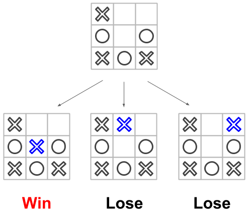
Here, you can see the position as the vertex and the changes in the position as the edge. Now you know finding the path to win a tic-tac-toe game is kind of the graph search problem.
2. The algorithm of the breadth-first search
In the breadth-first search, we visit the vertex from around it and finally visit all vertices if possible. This is the actual algorithm as following.
1. Add the vertex to start the breadth-first search to the empty queue. Mark that vertex visited.2. Extract a vertex from the queue and add its neighbors to the queue if that isn’t marked visited.3. Repeat step 2 until the queue is empty.
Step 1 is initialization to execute the algorithm. Here when we add the vertex queue, we mark the vertex visited. Step 2 is the main process for the breadth-first search. Basically, this process repeats to add the neighbors of the vertex extracted from the queue to the queue. However, the vertices added to the queue are only marked not visited. I?ll explain the reason why we should do this later. Step 3 is the condition to finish the loop of step 2. When the queue is empty, we visited all reachable vertices from the vertex from which we start searching.
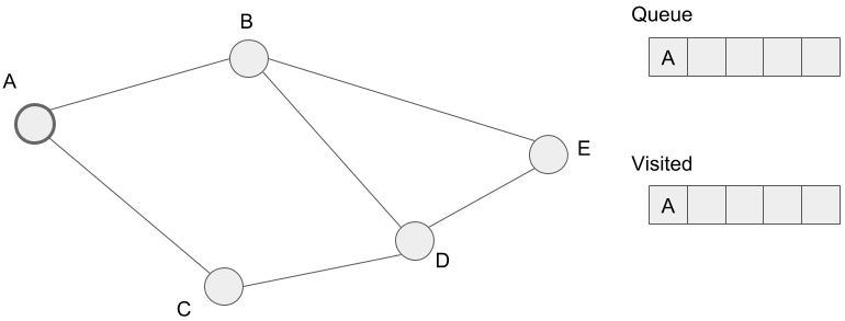
Let?s check the way how the algorithm works. In the graph below, we start searching from the vertex A. Here is the initial state below.
First, we extract vertex A from the queue. The neighbors of the vertex A, B and C, are not visited, so we add these to the queue.
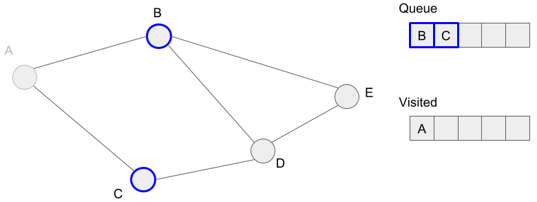
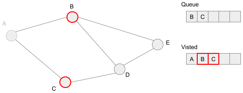
We mark the vertices, B and C as visited because we added these to the queue.
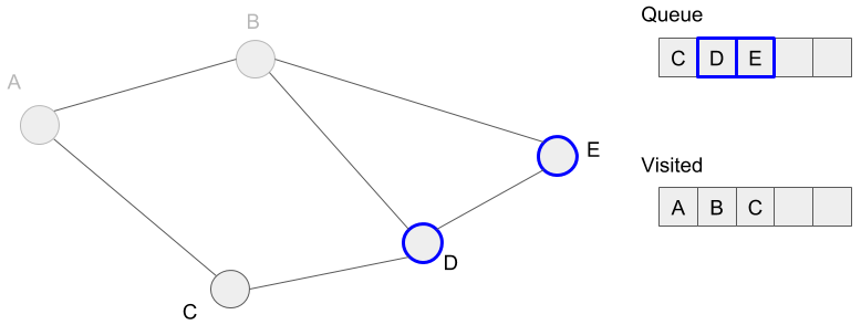
Next, we extract vertex B from the queue and then try to add the neighbors (A, D, E). However, we?ve already marked the vertex A as visited, so we only add the vertices D and E to the queue. Here, let?s think the case what if we also added the vertex A to the queue. If we add vertex A to the queue again, we should visit vertex A again. This means an infinite loop happens, so the program doesn?t finish. In other words, the condition of step 3 in the algorithm is always true because of the queue isn?t empty forever. This is the reason why we shouldn?t add the already visited vertex into the queue.
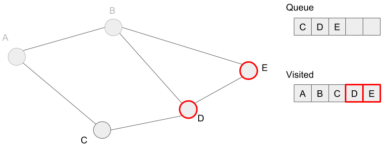
Then we mark vertices D and E visited because we added these to the queue.
We extract vertex C from the queue. However, we don?t have any vertex added to the queue because we?ve already visited all neighbors of vertex C.
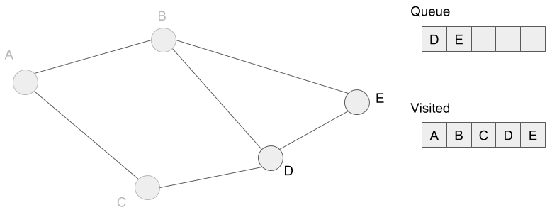
We are going to extract vertices D and E, but we?ve also visited these neighbors before. So the queue is empty and we finish to search. Finally, we?ve visited all reachable vertices from vertex A. In other words, we?ve marked all vertices visited.
3. Shortest path
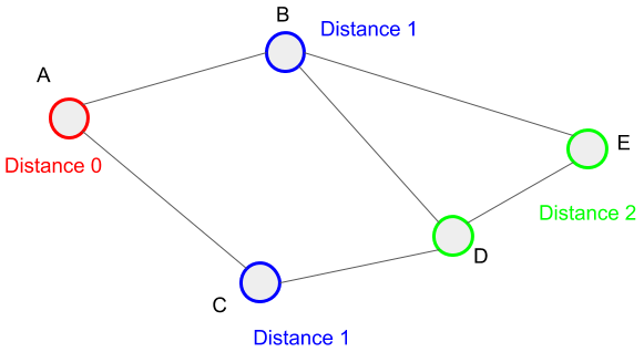
In the previous section, we?ve seen the way to visit all reachable vertices from vertex A. Here, we?ll look at the distance and the path from vertex A to one vertex. All paths derived by the breadth-first search are the shortest paths from the starting vertex to the ending vertices.
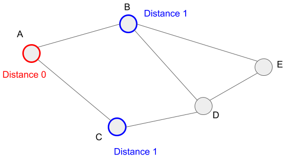
Let?s check this in the graph below. In the breadth-first search, we visited vertices B and C first. This means that we add B and C to the queue first and the timing to add in step 2 of the algorithm is the same. This tells us we can visit vertices B and C from vertex A at 1 distance. Please note that 1 distance is 1 edge in this case. Also, the paths from vertex A to vertices B and C are A to B and A to C respectively.
Then in the breadth-first search, we extracted vertex B from the queue and added its neighbors to the queue. In this time, we can reach vertices D and E from vertex A at 2 distances. This is because we can reach vertices D and E from vertex B at 1 distance and also vertex B from vertex A at 1 distance. The paths to reach vertices D and E are A to B to D and A to B to E respectively.
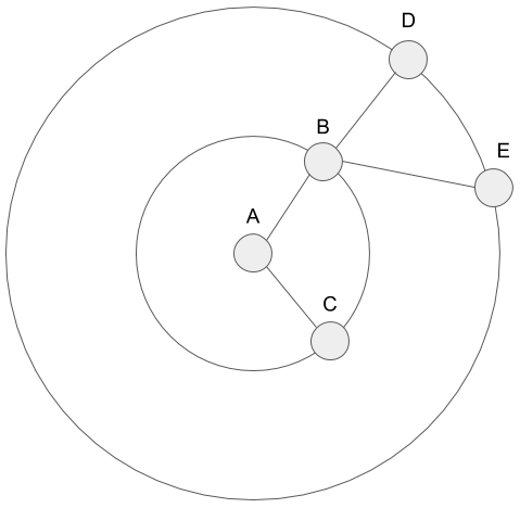
Here the important thing is that the paths derived from the breadth-first search are the shortest path from the vertex to some vertices. In the breadth-first search, we repeat the operation to visit vertices at 1 distance, 2 distance, and so on. So we get this result. We can say that we visit the vertices inside the circle of radius 1, radius 2, and so on in the breadth-first search like the figure below.
Someone think the shortest path to vertex D can be either A to B to D or A to C to D. In the breadth-first search if the distance to one vertex is the same, the path to the vertex will be changed by the order to extract a vertex from the queue. We add vertices in alphabetical order so far. For example, if we have vertices B and C to add, we add vertex B to the queue first.

In the breadth-first search, we don?t need to care the order of adding a vertex to the queue if the timing to add is the same. So we can add vertex C to the queue first in the example above. In this case, the path to vertex D is A to C to D. In summary, the difference between A to B to D and A to C to D depends on the order to add the vertex to the queue. So we can derive the shortest paths from one vertex to the other reachable vertices in the breadth-first search and one path is picked if there are the multiple shortest paths.
4. The implementation of the breadth-first search
The implementation with Python will be as follow. I?ll explain it line by line.
from collections import dequedef bfs(graph, vertex): queue = deque([vertex]) visited = {vertex: True} while queue: v = queue.popleft() for n in graph[v]: if n not in visited: queue.append(n) visited[n] = True
Following two lines initialize variables to start the breadth-first search. These lines prepare the queue and the visited.
queue = deque([vertex])visited = {vertex: True}
Next, the inside of the while-loop below is the main processing of the breadth-first search. Here graph[v] returns neighbors of vertex v.
v = queue.popleft()for n in graph[v]: if n not in visited: queue.append(n) visited[n] = True
This program extracts a vertex from the queue and adds its neighbors not marked visited the queue. It repeats this operation until the queue is empty.
However, we cannot know a distance or a path from the program above. So I?ll change the program slightly like below.
from collections import dequedef bfs(graph, vertex): queue = deque([vertex]) level = {vertex: 0} parent = {vertex: None} while queue: v = queue.popleft() for n in graph[v]: if n not in level: queue.append(n) level[n] = level[v] + 1 parent[n] = v return level, parent
I changed the initialization part. I added the level and the parent instead of the visited.
queue = deque([vertex])level = {vertex: 0}parent = {vertex: None}
The level holds distances from the vertex from which we start searching. The distance from the vertex to itself is 0, of course, we initialize the level above. The parent holds the vertex just added as a key and the vertex from which we reach to the vertex just added as a value. I?ll explain the reason why we need it later.
Then let?s look at the changes in the inside of the while loop.
for n in graph[v]: if n not in level: queue.append(n) level[n] = level[v] + 1 parent[n] = v
The level plays a role of the visited before. Also, we need to increment the i after the for-loop finishes because we need to expand the circle to search.
By using the parent, we can know the path to some vertex. I?ll explain this through the example. First, let?s think about the familiar graph below we use it a lot in this post.
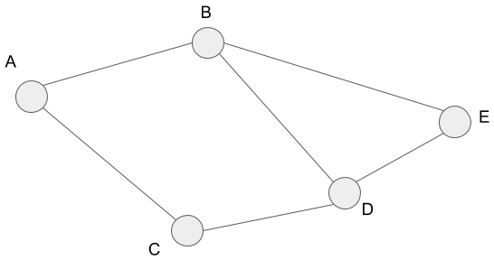
We can express the graph above as follows.
graph = { ‘A’: [‘B’, ‘C’], ‘B’: [‘A’, ‘D’, ‘E’], ‘C’: [‘A’, ‘D’], ‘D’: [‘B’, ‘C’, ‘E’], ‘E’: [‘B’, ‘D’]}
The key express the vertex and the value express its neighbors. We apply the breadth-first search to vertex A in this graph and get this result:
({‘A’: 0, ‘B’: 1, ‘C’, 1, ‘D’: 2, ‘E’, 2}, # level {‘A’: None, ‘B’: ‘A’, ‘C’: ‘A’, ‘D’, ‘B’, ‘E’, ‘B’}) # parent
The level has distances from vertex A. The parent means the figure below.
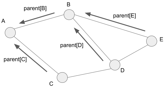
As the figure shows, we can know the path by tracing the parent. For instance, we can get the path from vertex A to vertex E by tracing the parent[E], parent[parent[E]], and so on. We should stop tracing when the parent returns vertex A. Finally, we get the path by reversing the result.
5. The time complexity of the breadth-first search
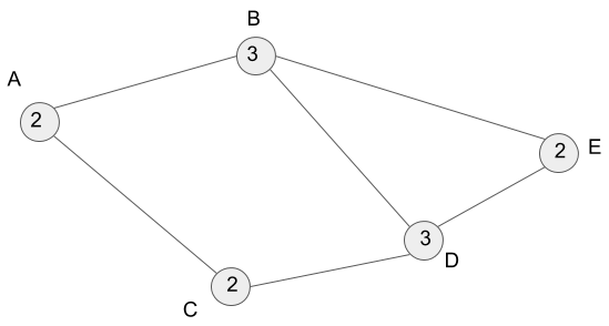
5.1 Degree in graph theory
In this section, I?ll explain the degree for you to understand the time complexity of the breadth-first search. We define the degree for a vertex on an undirected graph and the degree stands the number of the vertex?s neighbors. We express the degree as deg(v). For the figure below, deg(A) is 2 because vertex A is adjacent to vertices B and C. I show the degrees for each vertex as follows.
Also, the sum of all the degrees of the vertices become:

The sum of all the edges is 6. In an undirected graph, we count the edges twice when we compute the degree. So the sum of all the degrees alway doubles as the sum of all edges. Therefore, we obtain the following equation:

This is called handshaking lemma. Please note that V is the set of the vertices and E is the set of the edges.
5.2 Time complexity
Let?s think about the time complexity of the breadth-first search. Here we use an adjacent list to express a graph. The following part of the breadth-first search affects the time complexity.
while queue: v = queue.popleft() for n in graph[v]: if n not in level: queue.append(n) level[n] = level[v] + 1 parent[n] = v
This is because we take O(1) time for initialization, adding an item to the queue, extracting an item from the queue and marking the vertex visited. So we can obtain the time complexity by counting the number to visit the vertices. The number to visit the vertices will be the sum of repeats in the while-loop and the for-loop.
The repeats in the while-loop become |V| in the worst case. Here we assume the set of vertices V. The repeats will be the sum of the vertices at most because we only add the vertices not visited. The repeats in the for-loop become 2|E| in the worst case. Here we assume the set of edges E. The repeats in the only one for-loop will be the degree. So the repeats in all for-loop will be the sum of the degrees. By handshaking lemma, the sum is 2|E|. Therefore, we get the time complexity of the breadth-first search as O(|V|+|E|).
6. Conclusion
In this post, I explain the algorithm, the time complexity, and the Python implementation in the breadth-first search which is important for competitive programming. We need to keep the shortest path derived from the breadth-first search in mind. That?s all. Thank you for reading my article.
References
- MIT OpenCourseWare 6.006 Lecture 13: Breadth-First Search (BFS)
- MIT OpenCourseWare 6.006 Recitation 13: Breadth-First Search (BFS)

