Building an autoencoder model for reconstruction
 Logo retrieved from Wikimedia Commons.
This is the PyTorch equivalent of my previous article on implementing an autoencoder in TensorFlow 2.0, which you may read through the following link,
Implementing an Autoencoder in TensorFlow 2.0
by Abien Fred Agarap
towardsdatascience.com
First, to install PyTorch, you may use the following pip command,
pip install torch torchvision
The torchvision package contains the image data sets that are ready for use in PyTorch.
More details on its installation through this guide from pytorch.org.
Autoencoder
Since the linked article above already explains what is an autoencoder, we will only briefly discuss what it is.
An autoencoder is a type of neural network that finds the function mapping the features x to itself. This objective is known as reconstruction, and an autoencoder accomplishes this through the following process: (1) an encoder learns the data representation in lower-dimension space, i.e. extracting the most salient features of the data, and (2) a decoder learns to reconstruct the original data based on the learned representation by the encoder.
Mathematically, process (1) learns the data representation z from the input features x, which then serves as an input to the decoder.
 z is the learned data representation by the encoder f(h(x)) from input data x.
Then, process (2) tries to reconstruct the data based on the learned data representation z.
 x-hat is the reconstructed data by the decoder f(h(z)) based on the learned representation z.
The encoder and the decoder are neural networks that build the autoencoder model, as depicted in the following figure,
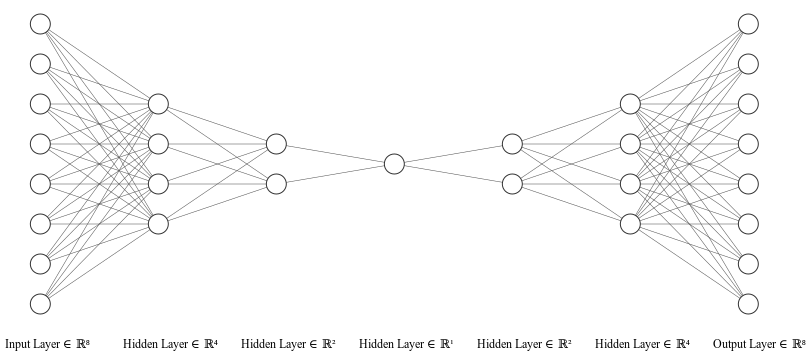 Illustrated using NN-SVG. An autoencoder is an artificial neural network that aims to learn how to reconstruct a data.
To simplify the implementation, we write the encoder and decoder layers in one class as follows,
The autoencoder model written as a custom torch.nn.Module.
Explaining some of the components in the code snippet above,
- The torch.nn.Linear layer creates a linear function (?x + b), with its parameters initialized (by default) with He/Kaiming uniform initialization, as it can be confirmed here. This means we will call an activation/non-linearity for such layers.
- The in_features parameter dictates the feature size of the input tensor to a particular layer, e.g. in self.encoder_hidden_layer, it accepts an input tensor with the size of [N, input_shape] where N is the number of examples, and input_shape is the number of features in one example.
- The out_features parameter dictates the feature size of the output tensor of a particular layer. Hence, in the self.decoder_output_layer, the feature size is kwargs[“input_shape”], denoting that it reconstructs the original data input.
- The forward() function defines the forward pass for a model, similar to call in tf.keras.Model. This is the function invoked when we pass input tensors to an instantiated object of a torch.nn.Module class.
To optimize our autoencoder to reconstruct data, we minimize the following reconstruction loss,
 The reconstruction error in this case is the mean-squared error function that you?re likely to be familiar with.
We instantiate an autoencoder class, and move (using the to() function) its parameters to a torch.device, which may be a GPU (cuda device, if one exists in your system) or a CPU (lines 2 and 6 in the code snippet below).
Then, we create an optimizer object (line 10) that will be used to minimize our reconstruction loss (line 13).
Instantiating an autoencoder model, an optimizer, and a loss function for training.
For this article, let?s use our favorite dataset, MNIST. In the following code snippet, we load the MNIST dataset as tensors using the torchvision.transforms.ToTensor() class. The dataset is downloaded (download=True) to the specified directory (root=<directory>) when it is not yet present in our system.
Loading the MNIST dataset, and creating a data loader object for it.
After loading the dataset, we create a torch.utils.data.DataLoader object for it, which will be used in model computations.
Finally, we can train our model for a specified number of epochs as follows,
Training loop for the autoencoder model.
In our data loader, we only need to get the features since our goal is reconstruction using autoencoder (i.e. an unsupervised learning goal). The features loaded are 3D tensors by default, e.g. for the training data, its size is [60000, 28, 28]. Since we defined our in_features for the encoder layer above as the number of features, we pass 2D tensors to the model by reshaping batch_features using the .view(-1, 784) function (think of this as np.reshape() in NumPy), where 784 is the size for a flattened image with 28 by 28 pixels such as MNIST.
At each epoch, we reset the gradients back to zero by using optimizer.zero_grad(), since PyTorch accumulates gradients on subsequent passes. Of course, we compute a reconstruction on the training examples by calling our model on it, i.e. outputs = model(batch_features). Subsequently, we compute the reconstruction loss on the training examples, and perform backpropagation of errors with train_loss.backward() , and optimize our model with optimizer.step() based on the current gradients computed using the .backward() function call.
To see how our training is going, we accumulate the training loss for each epoch (loss += training_loss.item() ), and compute the average training loss across an epoch (loss = loss / len(train_loader)).
Results
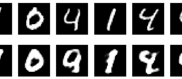
For this article, the autoencoder model was trained for 20 epochs, and the following figure plots the original (top) and reconstructed (bottom) MNIST images.
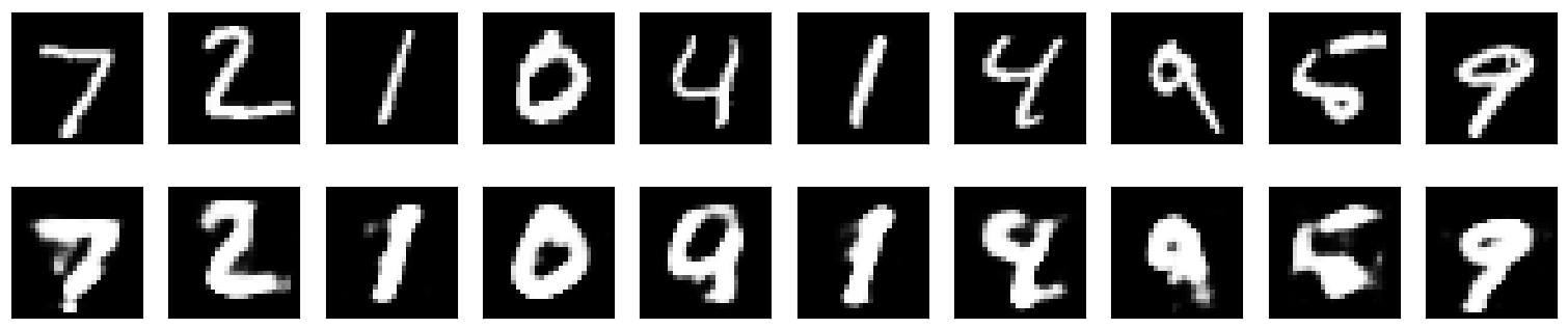 Plotted using matplotlib. Results on MNIST handwritten digit dataset. Images at the top row are the original ones while images at the bottom row are the reconstructed ones.
In case you want to try this autoencoder on other datasets, you can take a look at the available image datasets from torchvision.
Closing Remarks
I hope this has been a clear tutorial on implementing an autoencoder in PyTorch. To further improve the reconstruction capability of our implemented autoencoder, you may try to use convolutional layers (torch.nn.Conv2d) to build a convolutional neural network-based autoencoder.
The corresponding notebook to this article is available here. In case you have any feedback, you may reach me through Twitter.
References
- A.F. Agarap, Implementing an Autoencoder in TensorFlow 2.0 (2019). Towards Data Science.
- I. Goodfellow, Y. Bengio, & A. Courville, Deep learning (2016). MIT press.
- A. Paszke, et al. PyTorch: An imperative style, high-performance deep learning library (2019). Advances in Neural Information Processing Systems.
- PyTorch Documentation. https://pytorch.org/docs/stable/nn.html.

