Normalization is a technique often applied as part of data preparation for machine learning. The goal of normalization is to change the values of numeric columns in the dataset to a common scale, without distorting differences in the ranges of values. For machine learning, every dataset does not require normalization. It is required only when features have different ranges.
For example, consider a data set containing two features, age(x1), and income(x2). Where age ranges from 0?100, while income ranges from 0?20,000 and higher. Income is about 1,000 times larger than age and ranges from 20,000?500,000. So, these two features are in very different ranges. When we do further analysis, like multivariate linear regression, for example, the attributed income will intrinsically influence the result more due to its larger value. But this doesn?t necessarily mean it is more important as a predictor.
To explain further let’s build two deep neural network models: one without using normalized data and another one with normalized data and at the end, I will compare the results of these 2 models and will show the effect of normalization on the accuracy of the models.
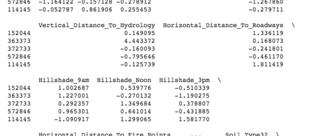
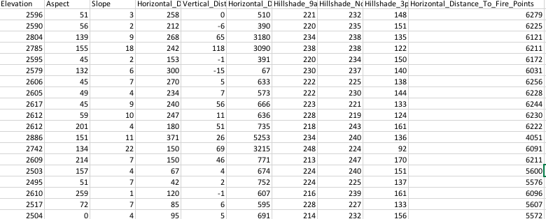 First Few Rows Of Original Data
Below is a Neural Network Model built using original unnormalized data:
”’Using covertype dataset from kaggle to predict forest cover type”’#Import pandas, tensorflow and kerasimport pandas as pdfrom sklearn.cross_validation import train_test_splitimport tensorflow as tffrom tensorflow.python.data import Datasetimport kerasfrom keras.utils import to_categoricalfrom keras import modelsfrom keras import layers#Read the data from csv filedf = pd.read_csv(‘covtype.csv’)#Select predictorsx = df[df.columns[:54]]#Target variable y = df.Cover_Type#Split data into train and test x_train, x_test, y_train, y_test = train_test_split(x, y , train_size = 0.7, random_state = 90)”’As y variable is multi class categorical variable, hence using softmax as activation function and sparse-categorical cross entropy as loss function.”’model = keras.Sequential([ keras.layers.Dense(64, activation=tf.nn.relu, input_shape=(x_train.shape[1],)), keras.layers.Dense(64, activation=tf.nn.relu), keras.layers.Dense(8, activation= ‘softmax’) ])model.compile(optimizer=tf.train.AdamOptimizer(), loss=’sparse_categorical_crossentropy’, metrics=[‘accuracy’])history1 = model.fit( x_train, y_train, epochs= 26, batch_size = 60, validation_data = (x_test, y_test))Output:Epoch 1/26 406708/406708 [==============================] ? 19s 47us/step ? loss: 8.2614 ? acc: 0.4874 ? val_loss: 8.2531 ? val_acc: 0.4880Epoch 2/26 406708/406708 [==============================] ? 18s 45us/step ? loss: 8.2614 ? acc: 0.4874 ? val_loss: 8.2531 ? val_acc: 0.4880?……………Epoch 26/26 406708/406708 [==============================] ? 17s 42us/step ? loss: 8.2614 ? acc: 0.4874 ? val_loss: 8.2531 ? val_acc: 0.4880
Validation accuracy of the above model is just 48.80%.
Now lets first normalize the data and then build a deep neural network model. There are different methods to normalize data. I will be normalizing features by removing the mean and scaling it to unit variance.
from sklearn import preprocessingdf = pd.read_csv(‘covtype.csv’)x = df[df.columns[:55]]y = df.Cover_Typex_train, x_test, y_train, y_test = train_test_split(x, y , train_size = 0.7, random_state = 90)#Select numerical columns which needs to be normalizedtrain_norm = x_train[x_train.columns[0:10]]test_norm = x_test[x_test.columns[0:10]]# Normalize Training Data std_scale = preprocessing.StandardScaler().fit(train_norm)x_train_norm = std_scale.transform(train_norm)#Converting numpy array to dataframetraining_norm_col = pd.DataFrame(x_train_norm, index=train_norm.index, columns=train_norm.columns) x_train.update(training_norm_col)print (x_train.head())# Normalize Testing Data by using mean and SD of training setx_test_norm = std_scale.transform(test_norm)testing_norm_col = pd.DataFrame(x_test_norm, index=test_norm.index, columns=test_norm.columns) x_test.update(testing_norm_col)print (x_train.head())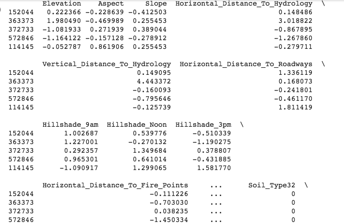 Output: Data after normalization#Build neural network model with normalized datamodel = keras.Sequential([ keras.layers.Dense(64, activation=tf.nn.relu, input_shape=(x_train.shape[1],)), keras.layers.Dense(64, activation=tf.nn.relu), keras.layers.Dense(8, activation= ‘softmax’) ])model.compile(optimizer=tf.train.AdamOptimizer(), loss=’sparse_categorical_crossentropy’, metrics=[‘accuracy’])history2 = model.fit( x_train, y_train, epochs= 26, batch_size = 60, validation_data = (x_test, y_test))#Output:Train on 464809 samples, validate on 116203 samples Epoch 1/26 464809/464809 [==============================] – 16s 34us/step – loss: 0.5433 – acc: 0.7675 – val_loss: 0.4701 – val_acc: 0.8022 Epoch 2/26 464809/464809 [==============================] – 16s 34us/step – loss: 0.4436 – acc: 0.8113 – val_loss: 0.4410 – val_acc: 0.8124 Epoch 3/26………………..Epoch 26/26 464809/464809 [==============================] – 16s 34us/step – loss: 0.2703 – acc: 0.8907 – val_loss: 0.2773 – val_acc: 0.8893
Validation accuracy of the model is 88.93%, which is pretty good.
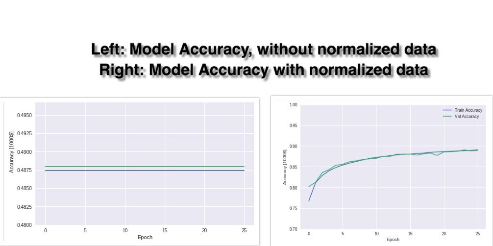 The accuracy plot of the above 2 models
From the above graphs, we see that model 1(left side graph) have very low validation accuracy (48%) and a straight line for accuracy is coming in a graph for both test and train data. Straight line for accuracy means that accuracy is not changing with the number of epochs and even at epoch 26 accuracy remains the same (what it was at an epoch 1). The reason for straight accuracy line and low accuracy is that the model is not able to learn in 26 epochs. Because different features do not have similar ranges of values and hence gradients may end up taking a long time and can oscillate back and forth and take a long time before it can finally find its way to the global/local minimum. To overcome the model learning problem, we normalize the data. We make sure that the different features take on similar ranges of values so that gradient descents can converge more quickly. From the above right-hand side graph, we can see that after normalizing the data in model 2 accuracy is increasing with every epoch and at epoch 26, accuracy reached 88.93%.
Thanks. Happy Learning 🙂

