 Not much for exciting leading images pertaining directly to Big O Notation, so a pensive puppy in the spirit of lighthearted seriousness.
What is Big O Notation?
It?s a way to draw insights into how scalable an algorithm is. It doesn?t tell you how fast or how slow an algorithm will go, but instead about how it changes with respect to its input size.
Literally, what does Big O mean?
Unlike Big ? (omega) and Big ? (theta), the ?O? in Big O is not greek. It stands for order. In mathematics, there are also Little o and Little ? (omega) notations, but mercifully they are rarely used in computer science and therefore out of scope here. All of these comprise a family of notations invented by Berlin-born mathematicians Paul Bachmann and Edmund Landau, and so you may also hear any of these referred to as Bachmann-Landau notations, or just Landau notations. Further these are also categorized as asymptotic notations, and you will probably most often hear them referred to as a set in this way. Complexity notation is another synonym you may encounter.
The Big Caveat
The important caveat is that Big O notation often refers to something different academically than it does in the industry, conversationally, in interviews, etc. In the wild, Big O actually often refers to what is academically known as Big ?. But for our illustrative purposes below, we?ll be using the academic definitions unless otherwise noted. Just remember that when you are talking Big O in real life, you?re mostly talking Big ?, or at least the most relevant Big O; this will all make sense in just a moment.
What do asymptotic notations do?
Asymptotic notations are super versatile and super cool. They measures how an algorithm scales in relation to its input size. Measuring as a functional relationship like this is crucial since if we were to measure concretely in units, say seconds or minutes, then we?d have to factor in all sorts of specific considerations like how fast a particular machine or compiler runs the algorithms. That would not be versatile or cool at all.
Asymptotic notations can be used to measure complexity not only in terms of runtime (time complexity), but also in terms resource requirements such as space on the call stack (space complexity). For simplicity sake, we?ll just discuss them in terms of runtimes here.
There are three asymptotic notations that programmers use: Big ? , Big ?, and Big O. Remember that in the field, Big O usually refers to Big ?. But let?s start with what Big O actually means.
What is Big O Notation?
Big O describes an upper bounding relationship. It is a function whose curve on a graph, at least after a certain point on the x-axis (input size), will always be higher on the y-axis (time) than the curve of the runtime. Since higher on the y-axis is more time, and therefore slower, the algorithm will always go faster, after a point, than the Big O.
That is hugely relevant for making analytical statements such as, ?well, in the worst case scenario (and often that is the expected case), my algorithm will scale at the very worst this quickly.? Or to say that another way: ?my algorithm will scale no more quickly (and therefore perform better) than this Big O does.? Or, ?my algorithm scales asymptotically no faster than this one.?
There is one important practical point to make at this point. In order for this to be conventionally relevant, you need to pick the closest possible Big O. For instance, if I have 9 dollars in my pocket, it is technically correct to say that I have no more than nine million dollars in my pocket. But that upper bound makes the statement functionally useless. It is more relevant to say that I have no more than 9 dollars in my pocket. We?ll get more into this later.
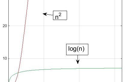
In the graph below, the green function is Big O of the red function. (That?s the case even though it?s a very weak Big O statement to make, as we?ll see.) It is written this way: green = O(red). That?s because green will always be lower/faster after a certain point on the x-axis (input size) than red. In this case, that point is right around 2.
Why do we say, at least after a certain point on the x-axis? That?s crucial. It?s because asymptotic notations are use to describe what happens with algorithms as the scale of their input sizes increase. In the graph above, the definition doesn?t care about the red algorithm actually being faster than the green one for inputs less than about 2, only that the nature of the relationship between the Big O curve and the runtime curve is that, after a certain point (around 2) and forever beyond that toward infinity, the Big O curve is greater.
Even if you run that red algorithm one billion times faster than the green one, eventually the red Big O curve will still overtake the green one, it?s just a matter of at how large an input size (and how far out we?d have to zoom the graph in order to see it). This is the nature of Big O, and we?ll illustrate it in a just a moment.
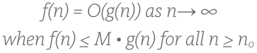
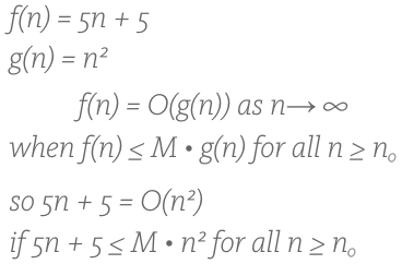
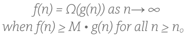
Don?t be put off by the equation below. It is the formal definition of Big O. It?s not that bad, seriously:
 Medium doesn?t have subscript formatting and therefore I can?t represent that last n in a paragraph except to call it ?n subscript o?, which I?ll do in the following paragraph.
In plain english it says: our runtime, which we call f(n), is Big O of g(n) if and only if there exists some constant M ? let?s make it 1 so that we don?t have to deal with it for now ? such that after some value of n, which the definition calls n subscript 0, g(n) will always be greater than f(n). n is the unit of the x axis, the input size. This is what we just saw in our last graph where n subscript 0 was about 2. The part with the infinity symbol just says that this occurs as n gets larger, or moves towards infinity. That?s it! We can pretty much simplify all that down to this:
?
How?s that? Remember for it to be Big O it doesn?t matter when the curves cross, so long as they do, and that after that, and forever, the curve of our function ? f(n) ? is always less than or equal to the Big O curve ? g(n). It?s that simple. Cool, right?
Why don?t we care when the lines cross, or about those relatively smaller values before the crossing point where the Big O line is actually below our function?s? Well we certainly would if we were planning on using input sizes in that range. But we?re also talking about scalability. We are interested in how things operate as they grow very large. That?s what Big O is for. For example:
5n + 5 = O(n)
In english, that is 5n + 5 is Big O of n, and therefore, at least after a certain value of n (input size), the curve of f(n), in this case 5n + 5, will always be overtaken by that of g(n), in this case n. In computer terms, this could mean that our algorithm runs 5 operations for every input (5n) and has a general setup or overhead of 5 regardless of the input size. Meanwhile, the Big O algorithm runs a nested for-loop which inspects an entire input array once for each element in the array. The graph looks like this:
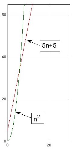
See how green overtakes red? See about where they cross? Let?s plug this into our formal definition:
So in simplest terms we pick 1 for M, since it can be any number, and we see below that when we plug in values the definition of Big O is satisfied because there is indeed a point ? in this case, between 5 and 6 ? beyond which the Big O curve becomes and forever remains greater (remember that means slower, since we are talking about greater amounts of time to run) than the curve of our original function. Therefore, in this case, our function is Big O, or ?, n:
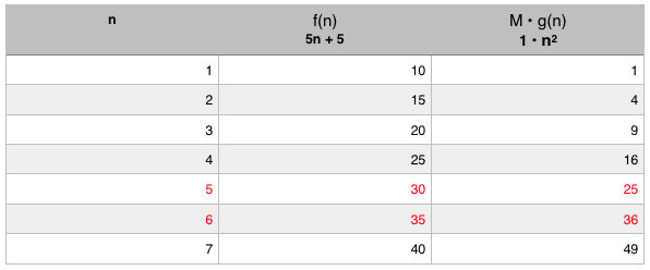 For input sizes less than 5, n is actually faster than 5n + 5. But at six and forever beyond, it is slower. That means it scales faster and that 5n + 5 = O(n).
Now, lets say we have a super computer that can run the faster scaling (gets slower for larger inputs) Big O algorithm ? g(n) or n in this case ? one thousand times faster than the computer running our original f(n) algorithm ? 5n+5. That would look like this:
The definition again.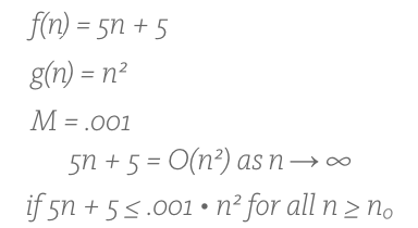 With our algorithms plugged in.
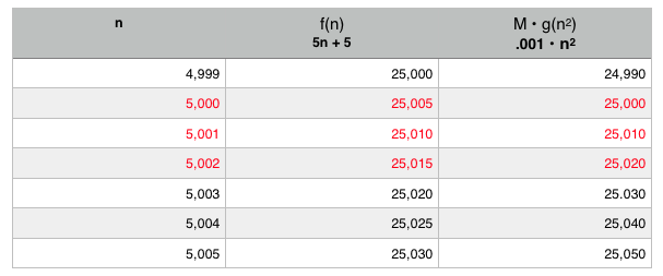
That .001 for M represents the g(n) function taking a thousandth of the time on our super computer. It may be a nice head start on the graph. But the beauty is that it doesn?t matter. That?s the crux of Big O. At some point, no matter how powerful the computer, no matter how nice the head start, the Big O line always overtakes, always scales faster, always becomes slower. It?s just a matter of when. That?s what Big O is. With this particular super computer its at an input size of around 5,001 (I rounded the below numbers for simplicity sake):
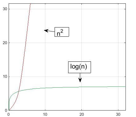
Keeping with this example, when we look at the graph on a small scale it looks like the Big O plot will never overtake our algorithm?s. But all we have to do is zoom out far enough to see that in fact it looks exactly the same regardless. And this will always be the case. Check out the graphs below:
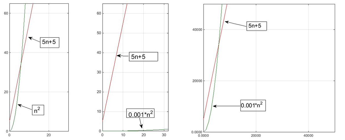
The first graph above is our original pair of algorithms graphed at our original scale. The second is the same scale, but with us running the green, less efficient algorithm 1000 times faster. Looking at that, it seems like it would never overtake our red algorithm. Instead, it appears here that green is now way faster and doesn?t really scale that quickly at all. But we know that?s not true because we have the power of our Big O understanding.
Now look at the third graph. Here we scale out far enough to see that Big O is always Big O, it?s just a matter of at what point. The input sizes are multiplied at this scale by 1000 too, and now we see that this graph looks identical to the first one even though the numbers are much much larger. We?re ok with how large the numbers are though because we use Big O notation when we want to know what happens when things get really big. That?s what we mean when we say Big O measures scalability.
Simplifying and Calculating Big O
A very important point from that last example is that the constants, and even the coefficients don?t really matter at scale. It?s plain to see that the constant 5 really isn?t important at all in 5n + 5. But even the coefficient 5 in the operand 5n can be ignored too. Eventually, no matter how you alter either algorithm (as we?ve just seen), a Big O with the dominant value n will always overtake one with the dominant value n.
Dominant values determine asymptotic notations because they set algorithms apart by the class of their growth rates. We can automatically drop that .001 too because it?s actually another coefficient. We showed how it didn?t matter at scale in that third graph.
Then we can say that the dominant value of 5n + n is n, and that the dominant value of .001 ? n is n, and therefore 5n + n is Big O of .001n, which is to say n = O(n). That is true, though it is still a weak Big O statement, since we?ll see later that any linear algorithm will always be Big O of any quadratic algorithm.
In real world terms, it?s easy to see how important this type of analysis can be. We saw in those graphs that even a one-thousand-times-slower computer will still perform better with its more efficient algorithm for all input sizes greater than about 5,001. That?s a pretty big deal!
Making it ?asier
The ??? symbol in plain english translates to ?is an element of?. For example: ?red ? color? means that red is an element of the set of colors. Or ?George Washington ? U.S. presidents? says that George Washington is a member of (or belongs to, or lies in, etc.) the collection of U.S. presidents.
Some people like to write their Big O notations like this, and I?m one of them:
n ? O(n)
That is nice compared with n = O(n) because all of the following (and an infinite many more) are also true:
n = O(n)
n = O(n?)
n = O(n? + 12)
Remember that if you have nine dollars in your pocket, it is technically less than nine hundred, nine million, etc. So the below notation is helpful in reminding us that in fact n is a member of the many functions which are Big O of n, and that it?s not a strict equivalency relationship.
n ? O(n)
The Best Big O
Given the above, the following, while technically accurate, is not the strongest Big O statement we can make:
n ? O(n)
But what is? Answer:
n ? O(n)
That may be irritating to you at first glance since in fact those are the same. But don?t get too aggravated yet! Remember the definition of Big O:
The key here is the M. If I have two algorithms on a graph with exactly the same curve (totally overlapping) but then multiply the second algorithm by any positive number, it will rise above the first. And then the lower function will have a Big O of the one above it. This is the closest possible Big O, and the strongest Big O statement we can make. It means that these two algorithms are in the same asymptotic class.
Big ?
Guess what? If you?ve got the Big O concept down, then you get Big Omega practically for free. It?s pretty much the exact same thing, just inverse. The formal definition is:
The only difference between the above and the Big O definition is the omega symbol and the greater than or equal to symbol (which was less than or equal to in Big O). In the same way we simplified that equation, we can do so here too:
?
Big Omega represents the fastest possible running time. It is a curve that lies below our function?s curve, at least after some point and forever toward infinity. A function will never perform faster (in less time) than it?s Big Omega.
Since miraculous streaks of best case scenarios are far more rare than worst case scenarios, which are often the average cases, it?s not hard to see why Big O is more popular than Big Omega.
Remember here too that, just as in Big O, there are weaker and stronger Big Omega statements. For instance, if Warren Buffett has a nine million dollar check in his hand, it isn?t a very strong, albeit true, statement to say that he holds a check for at least nine dollars.
Big ?
Big Theta is actually what most people are referring to when they talk about Big O. You?ll see why in just a minute. This is Big Theta:
f(n) = ?(g(n))
when f(n) = O(g(n))
AND f(n) = ?(g(n))
That means that one function is Big ? of another if and only if that function is both Big O and Big Omega of it. How can that happen? Let?s take a look at a formal definition of Big Theta:
g(n) ? k1 ? f(n) ? g(n) ? k2
In plain english, that says that f(n) is Big Theta of g(n) if and only if there exists at least two positive integers (k1 and k2) where the first one, when multiplied by g(n), will make its curve fall below that of f(n), and at the same time the second one multiplied by g(n) will make it go above.
If we can achieve this, then we?ve got the Big Theta, and that?s what is called a tight bound, an algorithm that bounds our own from both above and below. It will also represent the strongest possible asymptotic statement we can make.
For example, remember our strongest possible Big O statement:
n ? O(n)
This statement is true because if we multiply the Big O function by any number greater than 1, it will, at least after some point, forever be above the curve of our original function. It is the strongest Big O statement we can make. But wait, the opposite is true too. If we multiply it by a number less than 1, then at least after some point it will forever be below our original function. It?s also the strongest Big Omega statement we can make. Since both of these are true, so it is Big Theta!
n ? ?(n)
It is not always possible to make a Big Theta statement about an algorithm. But when it is, the Big Theta algorithm is in the same asymptotic class of algorithms as our own. It describes a tight bound and represents the strongest asymptotic statement we can make.
Big Due Diligence
There is a very small amount of memorization and a few great tips and tricks that can go a very long way in terms of working with Big O relationships.
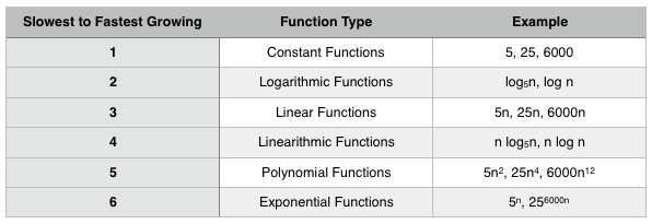
Below are function types in order of their growth rates from slowest to fastest growing. In other words, no matter what constants or coefficients there may be, these common algorithmic classes remain relative to each other in this order. So it?s a nice little cheat sheet:
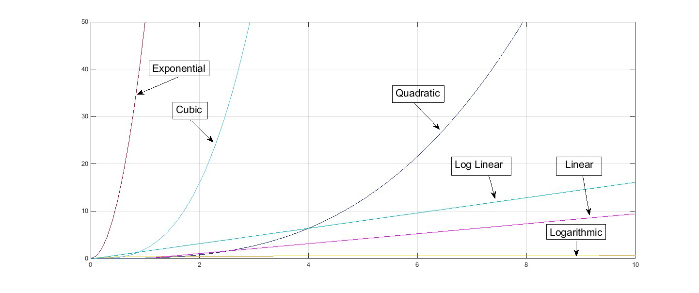
Here they are on a graph (constant would just be a straight horizontal line since it doesn?t grow at all):
So now that you know where a function stands categorically by type. There are some helpful reducing tricks to hone in on the Big O even more accurately within each class.
1. Get Rid of Constants and Coefficients
Remember how we should get rid of constants and coefficients? That?s the first trick. Get rid of them. (Though keep them in mind if you?re interested in when and how exactly a function may be overtaken by it?s Big O, or overtake its Big Omega.) Only the dominant terms are king. Here?s an example:

2. Combine Exponents and Know That The Larger Ones Scale Faster
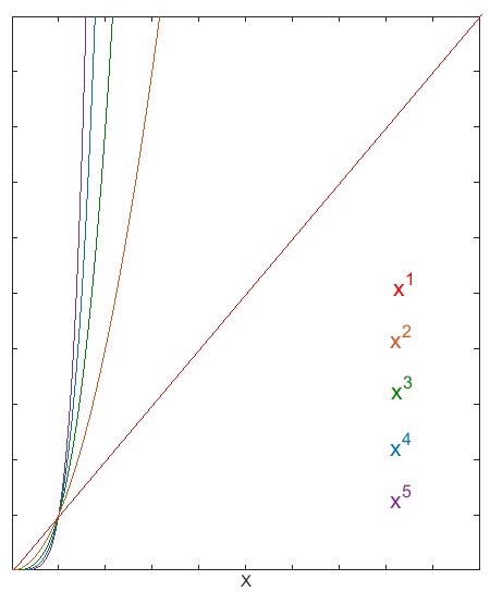
The above shows that a function scaling at O(n) is always above that of one scaling at O(n) (these are not Big Theta relationships). The same is always true for larger exponents. For example:
n ? O(n)
Also remember that you can combine exponents like this:

That?s because after dropping the constants and coefficients n ? n is n.
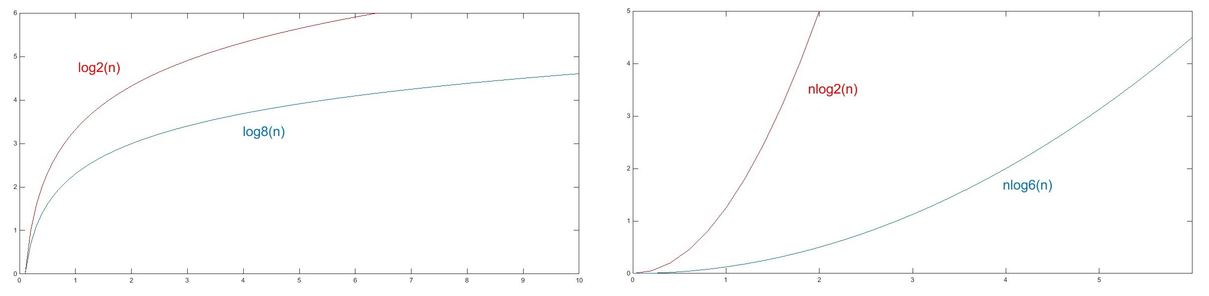
3. Know That All Log Bases Other Than 2 Can Be Simplified to Log Base 2, Yet Larger Ones Do Scale Faster (Both For Linearythmic and Logarithmic Functions)
This is true because of the mathematical formula below showing that, given a, b, and n are constants, log a of n and log b of n differ by log b of a, which is actually another constant, and therefor dropped:
![]()
Remember that though constants and coefficients have little bearing on asymptotic statements, they may actually come in handy if you are concerned with how and when the functions diverge. If that?s the case, then just as larger exponents grow faster than smaller ones, so logs with lesser bases grow more quickly than those with greater ones:
Other Big Os
Besides the common Big Os discussed here, know that there can be any number of others as unique as any of the algorithms they describe. The common list is not exhaustive but merely a helpful guide for learning. For instance, an algorithm with two inputs a and b may have a Big O of O(ab) or O(a+b) depending on how the inputs interact.
Should I use Big O to optimize every piece of code I write?
It?s helpful to remember that Big O, while a powerful tool for analyzing algorithms, isn?t the only consideration to be factored into the programming process. It may be tempting to use Big O prematurely or prioritize it too highly in a way that will overshadow other equally important considerations such as ?how easy is this code to work with and maintain?? In fact, all of the above doesn?t mean that an algorithm with a runtime of O(n) should never show up in your code.
Conclusion
Big O Notation provides programmers with an important tool for analyzing how algorithms scale.
The best two resources I?ve found on this subject are this lecture, and this one. They work nicely together as a pair.
If you don?t have a graphing program and want to play with one, I?ve used this one and you can use it too.
Related Reading Topic Recommendations
- Amortized Analysis
- Recursive Runtimes ? generally O(branches^depth)
- Factorials ? scale faster than all the common runtimes discussed

