
A Basic Overview & Visual Introduction To The Magic Of Waves

The Deep Study Of Nature Is The Most Fruitful Source Of Knowledge
It?s warmly appropriate that Jean-Baptiste Fourier left us with the poignant quote above as a stark reminder to continuously turn to our connection with nature as a source of inspiration for knowledge. It?s appropriate because, well, Fourier?s greatest contribution, the Fourier Series, both literally & figuratively, stems from a deep study of nature.
Literally, his key contribution to the annals of math history, the sole purpose of this exposition, came from the solution to a question posed by nature ? mainly, how does the temperature on a metallic plate distribute over time? How about at any given point on the plate? Figuratively, the search for the solution stemmed from a long-spanning tradition: our innate need to make sense of the world around us by describing it in terms of a circle.
Since ancient times, the circle was placed on a pedestal as the simplest shape for abstract comprehension. A simple center point & a fixed-length radius/string was all needed?every point on the perimeter perfectly equidistant from the center. The key to understanding the Fourier series (thus the Fourier transform & finally the Discrete Fourier Transform) is our ancient desire to express everything in terms of circles. The genius connection the rest of this piece revolves around, the heart of Fourier?s observation, stems from the elegantly-captivating realization below: from simple rotations in a circle we can create trigonometric functions of sine & cosine.
Introduction
As the term ?ancient? in the previous sentence implies, Jean-Baptiste Joseph Fourier (1768?1830 A.D.) was far from the first person to realize this. However, he was the first to cleverly note that multiple simple waves, either sine or cosine, could be added to perfectly duplicate any type of periodic function. More importantly, the series bears his name because he derived the ingenious method that reverse-engineered his observation: the Fourier Series setup & the required Fourier analysis is the process necessary to uncover all the sine & cosine waves that converge to a targeted function. Specifically, once setup, the analysis consists of deriving the coefficients (radius of) & frequencies (?speed? of rotation on) of the many circles whose summation mimics that of any generic periodic function.
The Fourier Series is the circle & wave-equivalent of the Taylor Series. Assuming you?re unfamiliar with that, the Fourier Series is simply a long, intimidating function that breaks down any periodic function into a simple series of sine & cosine waves. It?s a baffling concept to wrap your mind around, but almost any function can be expressed as a series of sine & cosine waves created from rotating circles. To give you an idea of just how pervasive this new perspective can be, take a look at the example below, where we outline a bird strictly using attached circles:
 Every circle rotating translates to a simple sin or cosine wave.
The larger implications of the Fourier Series, it?s application to non-periodic functions through the Fourier Transform, have long provided one of the principal methods of analysis for mathematical physics, engineering, & signal processing. The Fourier Series a key underpinning to any & all digital signal processing ? take a moment realize the breadth of this. Fourier?s work has spurred generalizations & applications that continue to develop right up to the present. As we?ll learn below, while the original theory of Fourier Series applies to periodic functions occurring in a natural wave motion, such as with light & sound, its generalizations, relate to significantly wider settings, such as the time-frequency analysis underlying the recent theories of wavelet analysis & local trigonometric analysis.
Post-Heat Equation
Baron Jean Baptiste Joseph Fourier (1768?1830) first introduced the idea that any periodic function can be represented by a series of sines & cosines waves in 1828; published in his dissertation Thorie analytique de la chaleur, which loosely translates to The Analytical Theory of Heat, Fourier?s work is a result of arriving at the answer to a particular heat equation. Panda the Red beautifully recounts this particular journey, as a result, we?re mainly focusing on everything post-heat equation discovery.
In short, from the heat equation, Fourier evolved his findings to develop the Fourier Series; since then, the Fourier Series has only increased in importance (though more through the Fourier Transform), particularly in the digital age. From creating the base for physics such as Brownian motion, for finance such as in the Black-Scholes equations, or for electrical engineering such as in digital processing, Fourier?s work has only grown in both theoretical & practical applications.
Since we?re covering Fourier Series here, however, our scope of work is slightly narrowed. Despite casually mentioning that the Fourier Series is only applicable to periodic function, the truth is a bit more nuanced.
Dirichlet Conditions
First, it must be noted that unlike the Fourier Transform, a Fourier Series cannot be applied to general functions ? they can only converge to periodic functions. Yet that?s not all, to guarantee a convergence of simple sine & cosine waves, three specific criteria must be met. Known as the Dirichlet conditions, named after one Peter Gustav Lejeune Dirichlet, all three conditions must be met for a periodic function with some period-length 2L:
- It has a finite number of discontinuities within the period 2L
- It has a finite average value in the period 2L
- it has a finite number of positive & negative maxima & minima
The three criteria above mainly ask: ?does the function have bounded variation?? If f(x) is periodic over the length of some period 2L, & checks-off each condition list above, then the Fourier Series guarantees that some mix of cosine & sine waves can replicate f(x). Next, we?ll dive into the Fourier Series itself ? starting from a very high level to working our way down to calculating exact coefficients.
Modern Fourier Series
An infinite series of numbers either goes to infinite or converges to a number, the same way an infinite series of expressions (either polynomials or trigonometric) either goes to infinite or converges to a function (or shape). Conversely, if we?re given a shape, we can approximate its function by creating an infinite series of varying sin & cosine waves.
The Fourier Series is simply a function that?s described & derived by a literal summation of waves & constants.
Formula Overview
We start with a high-level overview of the Fourier Series. Below, f(x) (left-side) is the target function we?re attempting to approximate through the Fourier Series (right-side):
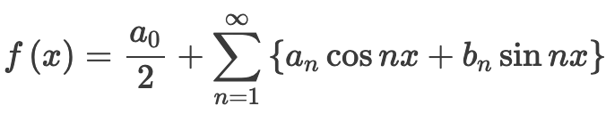
The ?Fourier Analysis? is simply the actual process of reverse-engineering, or constructing from scratch (sin & cos) a period function with the setup above ? the goal is to solve for coefficients a0, an & bn. The most commonly-seen notation for the Fourier Series looks like the above. Before we dive into the coefficients, let?s re-frame the above by explaining the two different parts.
f(x) = Avg. Function Value + Sine/Cosine Waves Series
The first part of the Fourier Series, the leading division that includes the coefficient a0 is simply the average value of the function; more specifically, it?s the net area between ?L & L, divided by 2L (the period of the function).
The second part of the equation, notated with a sigma/series symbol, represents the literal summation of different cosine & sines waves that should converge to target function; as one can tell, both trigonometric functions are carried to the nth-degree in the series. For this second half of the equation, the challenge is to solve for an & bn.
Fourier Analysis
As we head into the weeds of Fourier Analysis & we start to solve for our target coefficients (a0,an, & bn), there?s good news & bad news. The good news: there?s a standard setup for deriving all three coefficients as well as multiple short-cuts that we?ll introduce later on. The bad news: solving for a0,an & bn is straight-forward, yet far from simple. All three coefficients are solved through the following integrals:
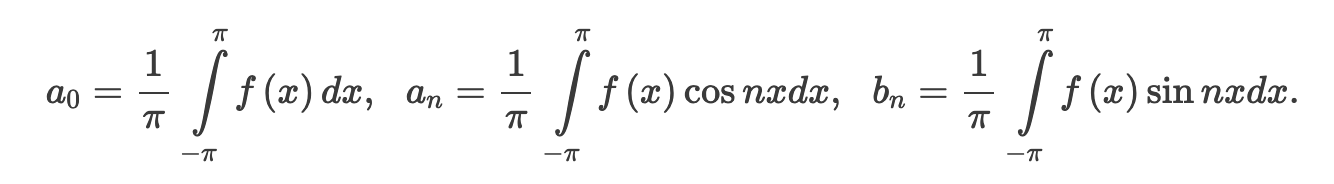 Note ? All Three Coefficients Given Assume A Set Period of 2?
Solving For a0 ? The Average Value
The first term on the left, a0 is at times referred to as the ?average value? coefficient for that very reason ? it?s simply an integral of the function we?re attempting to replicate over it?s fixed period.
Solving For aN? Summation of Cosine Waves
aN is the leading coefficient for the cosine waves in our series; our goal is to figure out how this coefficient behaves at different values in the series.
Solving For bN? Summation of Sine Waves
Conversely, bN is the leading coefficient for the sine waves in our series; our goal here is to again figure out how this coefficient behaves at different values in the series.
aN & bN are essentially the varying ?weights? of their respective waves ? they provide us with an approximation of which wave we?re ?mixing? in most for any given series.
Shortcuts ? Even & Odd Functions
Now, thankfully, most Fourier Series are drastically reduced in their complexity early-on; based on the symmetry of the target function f(x), whether the function is even or odd, we can usually eliminate at least one of the coefficients. For a review, it?s worth remembering that a function, relative to its symmetry across the origin or the y-axis, can be considered even or odd:
- F(x) is even if F(-x)=F(x), such as Cosine(x), F(x)*Cosine(x), etc?
- F(x) is odd if F(-x)=-F(x), such as Sine(x), F(x)*Sine(x), etc?
This section can make our lives a lot easier because it reduces the work required. The key shortcut here is to always start a Fourier analysis by first checking whether F(x), the function or shape we?re approximating, is odd, even or neither. If a function is odd or even, we?re in luck ? to recall some basic calculus, let?s remind ourselves what happens when we integrate either of the two trigonometric functions over some fixed period:
- The integral of Cos(x) from -L to L is 0
- The integral of Sin(x) from -L to L is also 0
Excellent ? with both sets of facts above, it?s clear now how a function?s symmetry drastically reduces its complexity for a Fourier Analysis; basically, in most, not all, problems that we encounter, the Fourier coefficients a0, aN or bN become zero after integration. With knowledge of even & odd functions, a zero coefficient is predicted without performing the integration, leading us to, essentially, a powerful shortcut. Let?s closely inspect both cases further.
Even Functions: Half-Range Fourier Cosine Series
A function F(x) is said to be even if F(-x) = F(x) for all values of x; therefore, the graph of an even function is always symmetrical about the y-axis (aka ? it is a mirror image). For example, take a look at the graph of the function below, F(x) = cos(?x):
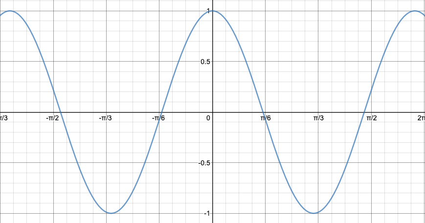 F(x) = Cos(?x)
Clearly, the above is symmetrical across the y-axis. If a function is even, then it follows that the integral part of solving for bN, no matter the nth-term of bN, is also equal to zero. Therefore, we can safely eliminate the bN part of our original series, leaving us with the truncated Fourier Series of an even function. Known as a Half-Range Fourier Cosine Series, it looks like the following:
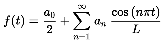
An even function has only cosine terms in its Fourier expansion: the key to understanding this & the following shortcut is the simple reminder that every Fourier Series setup starts with both a sine & a cosine function.
Odd Functions: Half-Range Fourier Sine Series
A function F(x) is said to be odd if F(-x) = -F(x) for all values of x; therefore, the graph of an odd function is always symmetrical about the origin (aka ? it?s unchanged when flipped over the x-axis & y-axis). For example, take a look at the graph of the function below, F(x) = sin(?x):
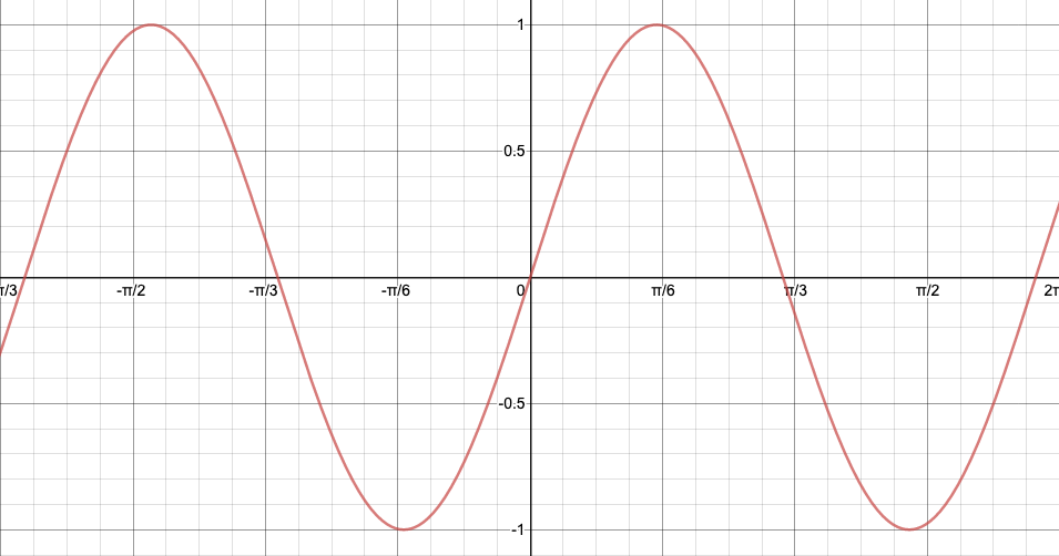 F(x) = Sin(?x)
It?s a bit harder to tell, but the above is symmetrical across the origin. If a function is odd, then it follows that the integral of the series terms including aN , no matter the nth-term of aN, is also equal to zero. Therefore, we can safely eliminate the aN part of our original series, leaving us with the truncated Fourier Series of an odd function; known as a Half-Range Fourier Sine Series. That?s not all, however, odd functions include extraneous information that helps us eliminate an additional term: a0. Think this through ? if a function is symmetrical across the origin, then this means that the area above the x-axis is equal to the area below the x-axis; which means that the average value of the function, our a0 term, is also equal to zero. Therefore, for a Half-Range Fourier Sine Series, we can safely eliminate both our first time a0 & our cosine term as such:
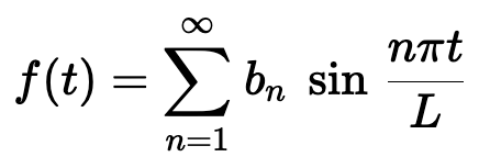
Much of the original setup now truncated, an odd function has only sine terms in its Fourier expansion; clearly, this is a significantly-simpler setup than our starting Fourier Series.
Examples
It?s now time to walk through an actual Fourier Series example! For this example, we?re going to replicate a square-wave that oscillates from troughs of -1 to crests of 1 with a period of 2?; we?re going to analyze the function from -? to ?-. This takes the following form (picture on the left/below).
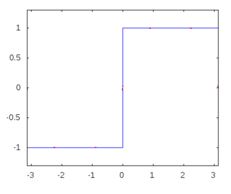 Note ? We?ve Remove The X/T & Y Axis
The very first step to setting up a Fourier Series is not to jump into the setup, but rather to check if the target function displays either type of symmetry; looking at the graph, it?s pretty clear that it is indeed symmetrical around the origin. Therefore, the function we?re working with is odd. That tiny piece of analysis drastically reduces the complexity & required steps to complete our Fourier Series. Since we know it?s an odd-function, this means we can treat it as a Half-Range Fourier Sine Series (described above). We start our actual journey through this example with the substantially-simpler setup:
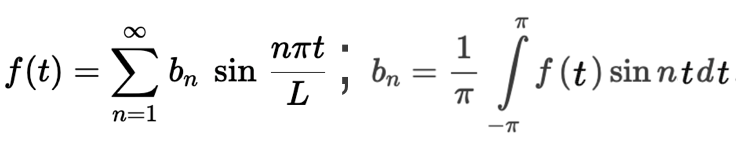 Our Goal Is To Solve for bN
Reading left-to-right, f(t) is the function we?re approximating with our Fourier series. As you can tell, we?ve already eliminated both the a0 & aN terms, we only have a series-sum of sine waves left to engineer. Past the semi-colon, to the right, we have the remaining coefficient that we need to solve.
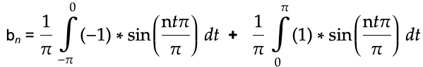
Here?s the part the tripped me up the first time: the f(t) on the right side is simply the value of the shape / function we?re approximating. In this particular example, as shown in the shape above, the value of the function f(t) is piecewise: from -? to 0, f(t) = -1; from 0 to ?, f(t) = 1. Therefore, if we split bN to two different integrations, (-?,0) to (0,?), we can simply substitute the f(t) variable with either -1 or 1:
Next, we work out a few sample values of n to analyze patterns that?ll hint to the convergence of our coefficient bN. Let?s start by writing out n = 1:
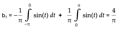
The above isn?t too complicated ? feel free to plug into wolfram alpha to double-check. It tells us though, that for the first value of n = 1, our coefficient of bN converges to the fraction 4/?. We?ll now repeat this process for four additional values of n in hopes of noticing a pattern:
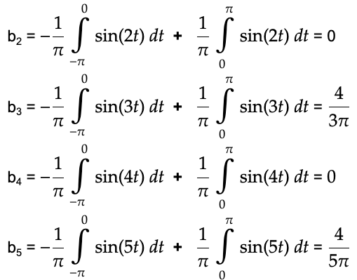
Is there a discernible pattern? Yes. Again, please double-check these piece-wise integrations with Wolfram Alpha or another advanced calculator. Looking at the above, it?s notable that all even values of bN converge to zero, while all the odd values of bN converge to: 4 / n*?.
With bN solved, we can now plug the coefficient back into our Half-Range Fourier Sine Series that we setup above. Let?s now write out the first few terms of our series below:
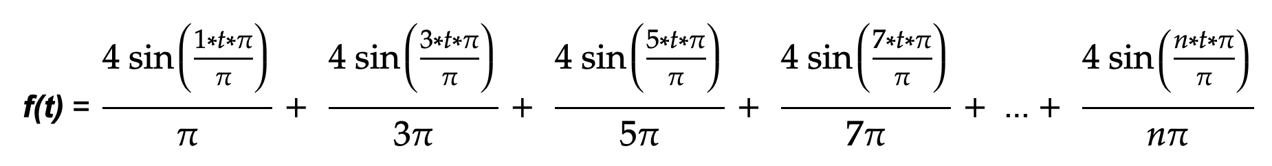
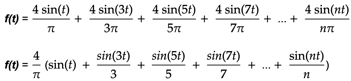
This is a bit convoluted, however, it?s already perfectly accurate: the Fourier Series on the right indeed converges to our target square-wave. We can further confirm this by simplifying & animating exactly how this convergence happens over time:
With our Fourier Series now properly solved, let?s take a quick moment to visually confirm what we solved. The animation below shows exactly how each of the terms above corresponds to a circle with a specific radius & frequency that, in summation, draw out our intended square graph:
Each circle has a different radius & frequency. Observable in the third column of the GIF above, by appending each circle at the end of the radius of the preceding circle, our wave gradually approaches a square wave. For a last & final check, we?re going to overlay the series as we approach infinity on top of the very initial opening graph:
I can?t think of a word more accurate to capture this than: beautiful. It?s simply captivating to watch in action & nothing short of rewarding to fully comprehend the underlying mechanics.
Onto Fourier Transforms
The Fourier Series is a way of representing periodic functions as an infinite sum of simpler sine & cosine waves. From signal processing to approximation theory to partial differential equations, it?s hard to overstate just how intricately the Fourier Series is tied with physics phenomena ? anything with an identifiable pattern can be described with varying sin & cosine waves.
Yet?that?s not the end of the story. As it?d turn out a few decades afterward, the scope of our Fourier Series is quite limited compared to its successor, the Fourier Transform. The Fourier Series is used to represent a periodic function by a discrete sum, while the Fourier Transform is used to represent a general, non-periodic function. The Fourier transform is essentially the limit of the Fourier series of a function as the period approaches infinity. At the heart of all digital-based technology, it?s the next stop on our journey for those curious to understand the nature of our everyday objects just a tad bit more.
This essay is part of a series of stories on math-related topics, published in Cantor?s Paradise, a weekly Medium publication. Thank you for reading!

