

Bayes? Theorem looks naively simple. We may model the prior and likelihood with known families of distribution. Therefore, the posterior equation is well-defined and we believe any calculations should be obvious.
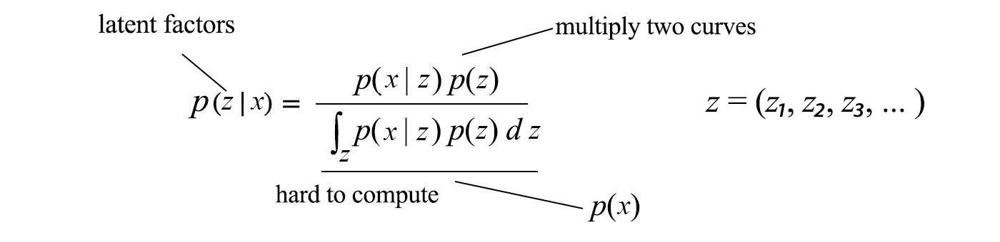
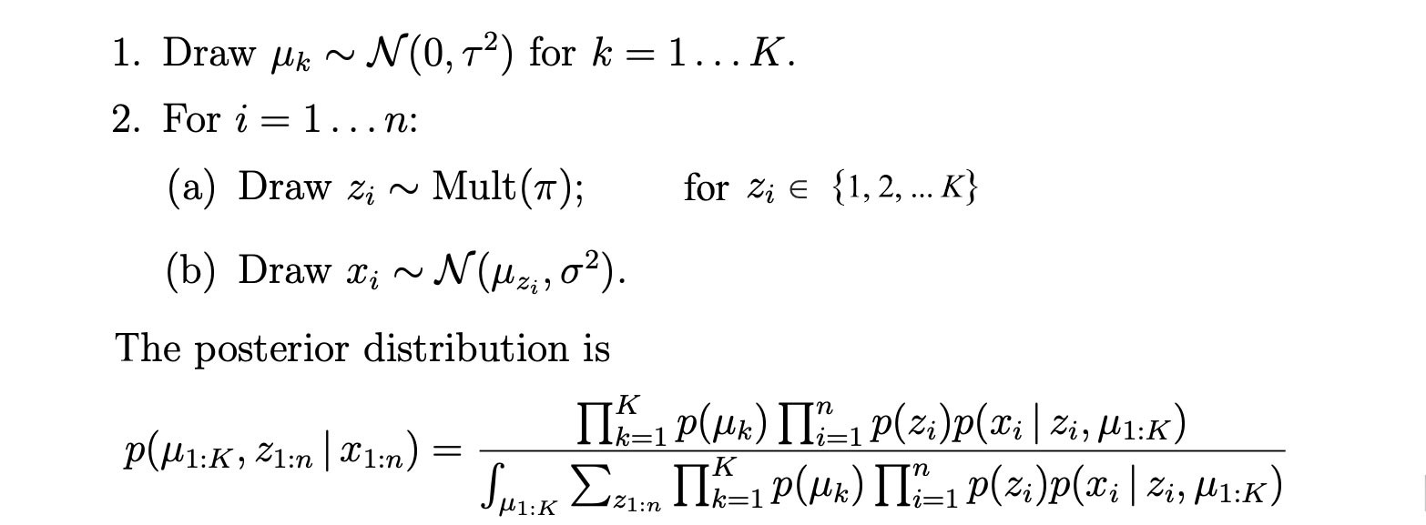
In reality, discover the latent variables z from the observation x is usually hard. Otherwise, AI problems can be solved easily. In the Bayes? Theorem, the denominator is the partition function which integrates over all variables composed of z. In general, this is intractable and cannot be solved analytically. Just as a demonstration, the following is a simple example in generating x? from one of the K normal distributions. As shown, the complexity of the posterior is not manageable.
 Modified from source
Even for some models, like the Bayesian network, the partition function equals to one. But analysis as simple as the expectation of p may remain intractable. Our alternative is to approximate the solution instead. In ML, there are two major approximation approaches. They are sampling and variational inference. In this article, we will discuss the latter.
In variational inferencing, we model the posterior directly. Given the observation X, we build a probability model q for latent variables z, i.e. q ?p(z|X).
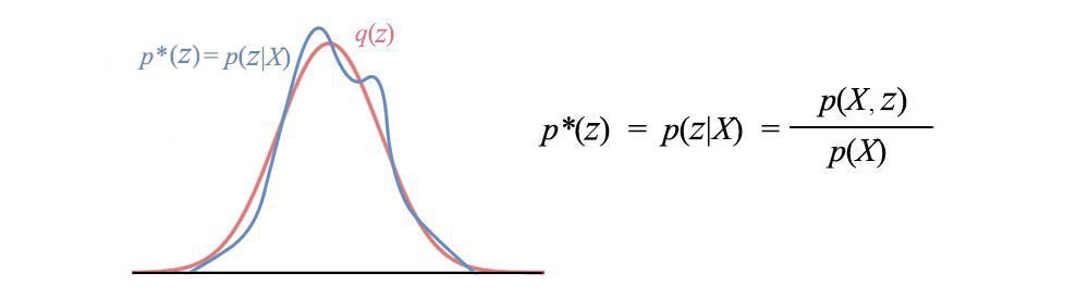
The marginal p(X) above can be computed as:

In variational inference, we avoid computing the marginal p(X). This partition function is usually nasty. Instead, we select some tractable families of distribution q to approximate p.

We fit q with sample data to learn the distribution parameters ?. When we make our choice for q, we make sure it is easy to manipulate. For example, its expectation and the normalization factor can be computed directly from the distribution parameters. Because of this choice, we can use q in place of p to make any inference or analysis.
Overview
While the concept sounds simple, the details are not. In this section, we will elaborate on the major steps with the famous topic modeling algorithm called Latent Dirichlet Allocation (LDA). We hope that this gives you a top-level overview before digging into the details and the proves.
The following is the Graphical model for LDA.
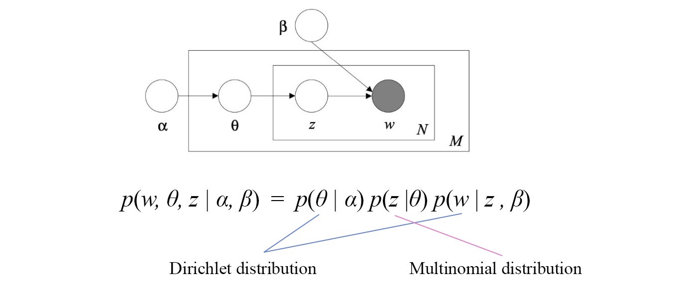
This model contains variable ?, ?, ?, z, and w. Don?t worry about the meanings of the variables since it is not important in our context. w is our observations. ? and z are the hidden variables (latent factors) that we want to discover. ? and ? are fixed and known in our discussion. The arrows in the Graphical model indicate dependence. For example, w depends on z and ? only. Hence, p(w|?, ?, ?, z) can be simplified to p(w|z, ?).
Like many probability models, we are interested in modeling the joint distribution p(w, ?, z |?, ?) for the observations and the unknowns. We apply the chain rule to expand the joint probability such that it composes of distributions of single variables only. Then, we apply the dependency from the graph to simplify each term. We get

Based on the topic modeling problem, ? and w can be modeled with Dirichlet distributions and z with a multinomial distribution. Our objective is to approximate p with q for all the hidden variables ? and z.

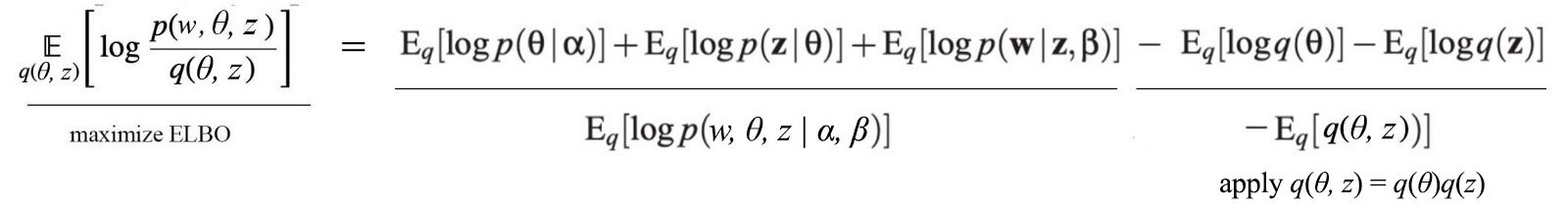
We define an objective to minimize the difference between p and q. This can be done as maximizing ELBO (Evidence Lower Bound) below.
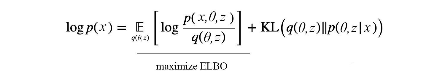
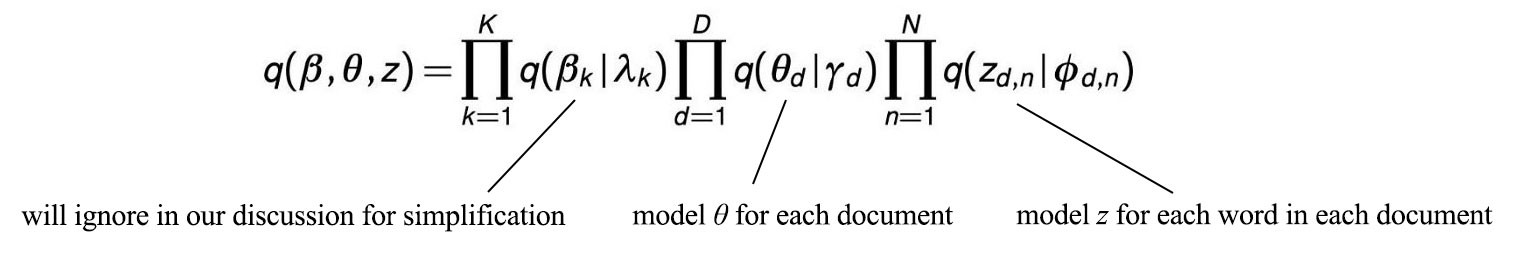
Even it is not that obvious, ELBO is maximized when p and q are the same. However, the joint probability q(?, z) is still too hard to model. We will break it up and approximate it as q(?, z) ? q(?) q(z). Even it may not be perfect, the empirical result is usually good. z composes of multiple variables z?, z?, z?, … and can be decomposed into individual components as q(z?)q(z?)… Therefore, the final model for q is:

According to the topic modeling problem, we can model ? with a Dirichlet distribution and z? with a multinomial distribution with ? and ?? for the corresponding distribution parameters. This is a great milestone since we manage to model a complex model with distributions of individual hidden variables and select a tractable distribution for each hidden variable. The remain question is how to learn ? and ??. Let?s get back to the ELBO objective:

In many ML problems, to model the problem effectively, hidden variables often depend on each other. We cannot optimize them in a single step. Instead, we optimize one variable at a time while holding other variables fixed. So, we rotate the hidden variables to be optimized in alternating steps until the solution converges. In LDA, z and ? are optimized in step 5 and 6 below separately.
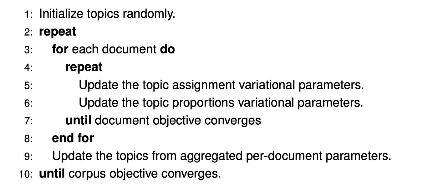 Source
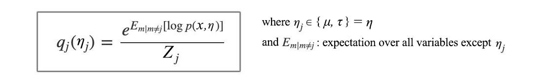
The remaining major question left is how to optimize a variational parameter while fixing others. In each iteration, the optimal distribution for the targeted hidden variable is:
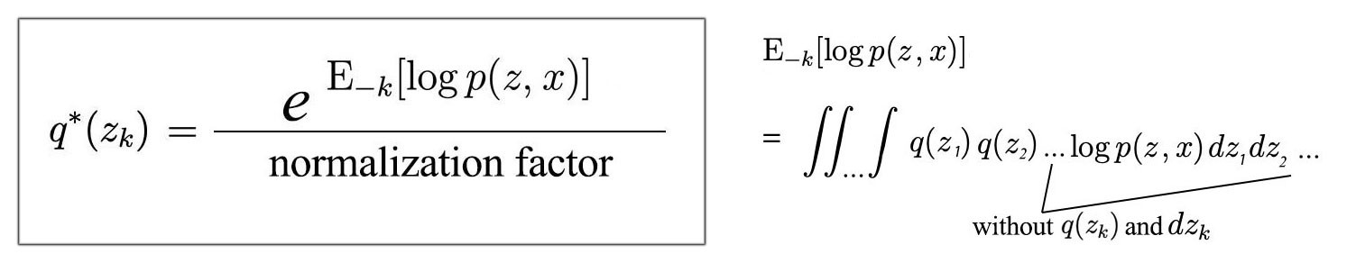
It sounds like we are reintroducing the evil twins back: the normalization factor. Nevertheless, it will not be a problem. We choose q to be tractable distributions. The expectation and the normalization can be derived from the distribution parameters analytically.
The numerator in the equation deserves more explanation. For a regular expectation E[f(x?, x?, x?)], we evaluate f over all variables.

But for our numerator, we omit the targeted variable.

i.e.,
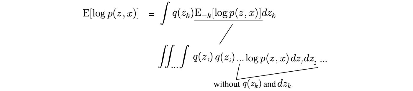
The -k is short for:

However, we will not perform the integration in computing the expectation. Our choice of q? allows us to simplify many calculations in the maximization of ELBO. Let?s detail it more.
In LDA, q is approximated as:
where ? and z are modeled by ? and ? respectively. Our calculation involves:
- Expand the ELBO into terms of individual variables
- Compute the expected value
- Optimize the ELBO
Expand ELBO
Using the Graphical model and the chain rule, we expand the ELBO as:
Compute the expected value
We don?t want to overwhelm you with details. Therefore, we only demonstrate how to compute the expectation for the first term only. First, ? is modeled by a Dirichlet distribution with parameter ?.
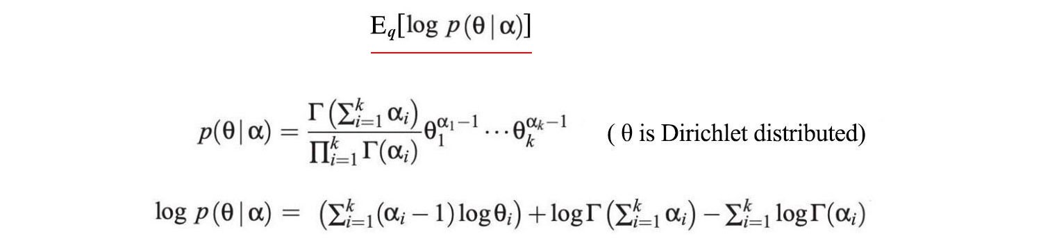
Next, we will compute its expectation w.r.t. q.
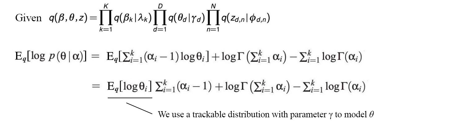
Without proof here, E[log ??] can be calculated directly from ?.
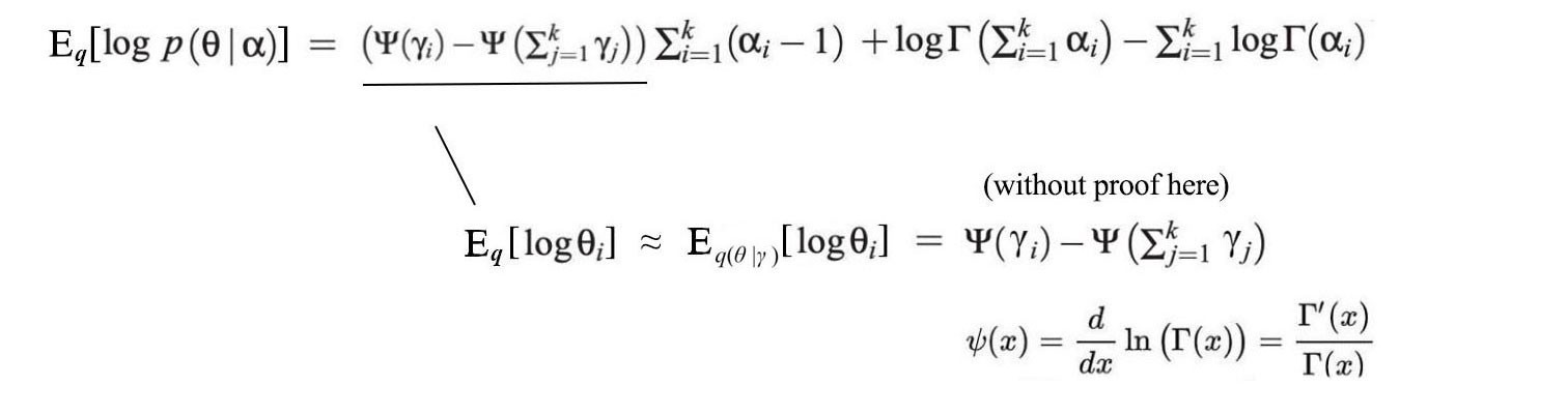
We choose q thoughtfully, usually with well-known distributions based on the property of the hidden variables in the problem statement. Mathematicians already solve those expectation expressions analytically. We don?t even worry about the normalization factor.
Optimize ELBO
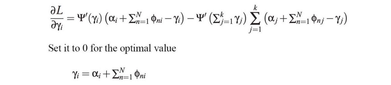
After we expand all the remaining terms in ELBO, we can differentiate it w.r.t. ?? (the ith parameter in ?) and ?n? (the ith parameter in nth word). By setting the derivative as zero, we find the optimal solution for ?? as:
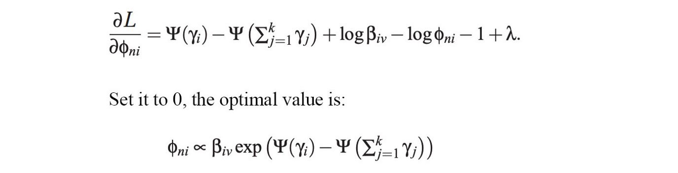
And the optimal solution for ?n? will be:
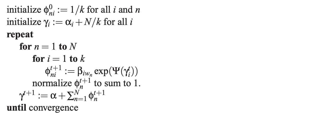
Because of the dependence between ? and ?n?, we will optimize the parameters iteratively in alternating steps.
 Source
Here is the overview. For the remaining of the articles, we will cover some major design decision in variational inference, proves and a detailed example.
KL-divergence
To find q, we turn the problem into an optimization problem. We compute the optimal parameters for q that minimizes the reverse KL-divergence for the target p*.

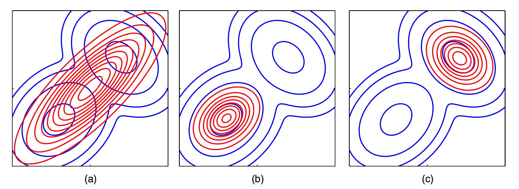
As shown before, KL-divergence is not symmetrical. The optimal solutions for q will only be the same for KL(p, q) and KL(q,p) when q is complex enough to model p. This raises an important question of why reverse KL-divergence KL(q,p) is used when KL-divergence KL(p, q) matches the expectation of p better. For example, when using a Gaussian distribution to model a bimodal distribution in blue, the reverse KL-divergence solutions will be either the red curve in the diagram (b) or (c). Both solutions cover one mode only.
 Source
However, the KL-divergence solution in (a) will cover most of the original distribution and its mean will match the mean of p*.
Moments, including the mean and the variance, describes a distribution. The KL-divergence solution is a moment projection (m-projection). It matches q with the moments of p. If we match all the moment parameters, they will be exactly the same. If a family of the exponential distribution is used for q, we can use KL-divergence to match the moments of q with p* exactly. Without much explanation here, their expected sufficient statistics will match.

(i.e. p=q) The reverse KL-divergence is an information projection (i-projection) which does not necessarily yield the right moments. Judged from this, we may conclude m-projection is superior. However, if a mechanism can match p* exactly, such a mechanism needs to understand p* fully too which is hard in the first place. So it does not sound as good as it may be.
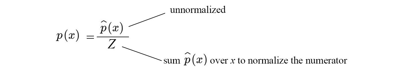
In variational inference, i-projection is used instead. To justify our choice, let?s bring up a couple of constraints that we want to follow. First, we want to avoid the computation of the partition function, the calculation is hard. Second, we want to avoid computing p(z) since we need the partition function to compute it. So let?s define a new term for p, the unnormalized distribution, that separate the partition function out.
Let?s plug the new definition into the reverse KL-divergence.
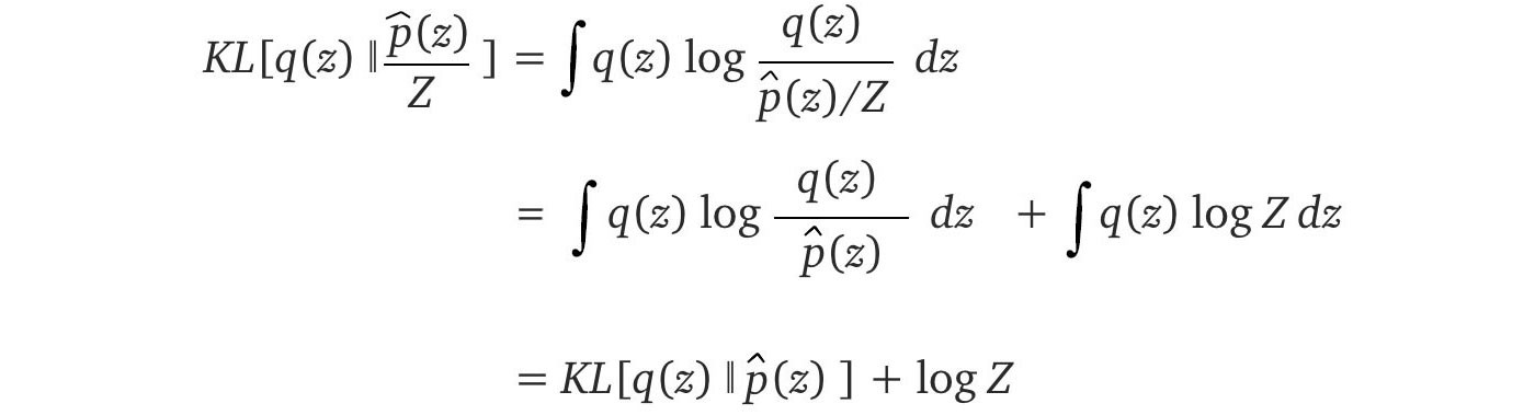
Z does not vary w.r.t. q. It can be ignored when we minimize reverse KL-divergence.

This is great news. In the Graphical model, the un-normalized p are well-defined using factors. They are easy to compute and the objective in the R.H.S. does not need any normalization. Using the reverse KL-divergence is a good compromise even it may not be perfect under certain scenarios. For q is overly simple compared with p*, the result may hurt. However, variation inference usually demonstrates good empirical results. Next, let?s see how to optimize the reverse KL-divergence.
Evidence lower bound (ELBO)
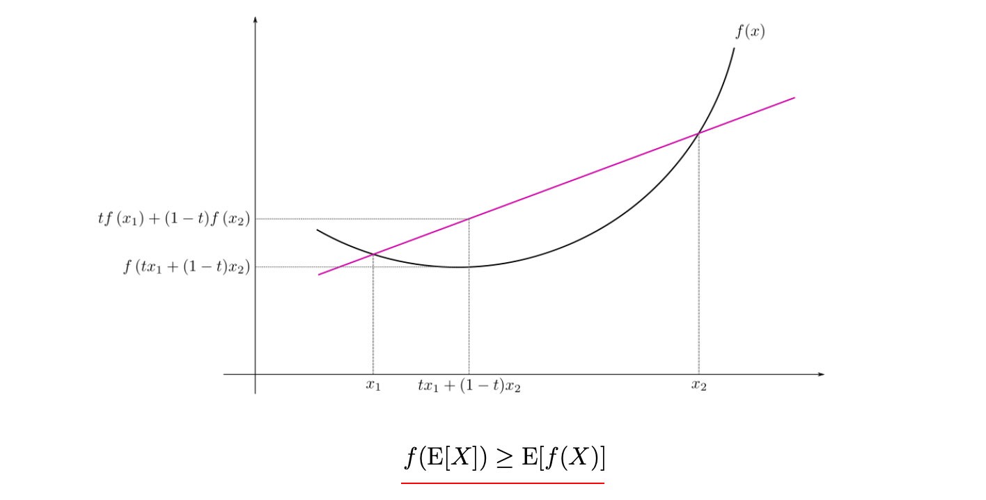
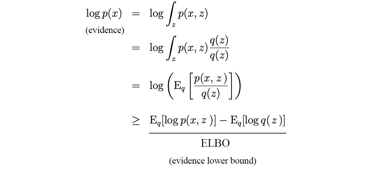
Let?s introduce the Jensen?s inequality below for a convex function f and a term called evidence lower bound (ELBO)
 The graph is originated from Wikipedia
ELBO is literally the lower bound of the evidence (log p(x)) after applying the Jensen?s inequality in the 4th step.
 Modified from source
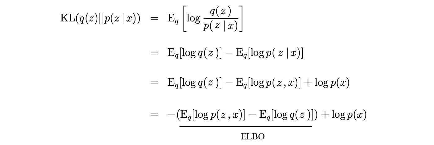
And ELBO is related to the KL-divergence as:
 Modified from source
Let Z be the marginal p(x) for now. Don?t confuse Z with the hidden variables z. Unfortunately, we need to overload the notation with a capital letter as Z is often used in other literature.

Z does not change on how we model q. So from the perspective of optimizing q, log Z is a constant.

Therefore, minimizing the KL-divergence will be the same as maximizing ELBO. Intuitively, given any distribution q, ELBO is always the lower bound for log Z. However, when q equals p*, the gap diminishes to zero. Therefore, maximizing ELBO reduce the KL-divergence to zero.
By maximizing the evidence lower bound ELBO, we minimize the difference of two data distributions.
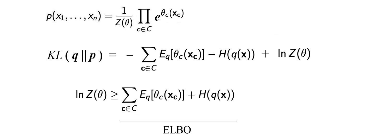
Let?s generalize the ELBO as
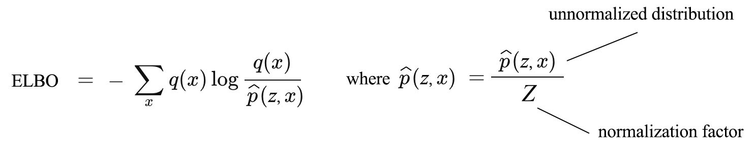
where Z is now a general normalization factor.
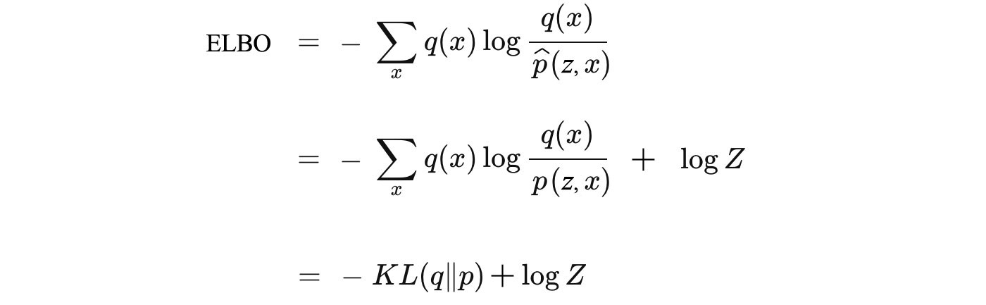
Again, as shown above, maximizing ELBO is the same as minimizing KL-divergence as Z does not vary on how we model q.

This brings a major advantage over the KL-divergence. ELBO works well for both normalized and unnormalized distribution and no need to calculate Z which is required for the regular KL-divergence definition.
ELBO and the Graphical model (optional)
Let?s demonstrate how the unnormalized distribution is computed in the ELBO using the Graphical model. The joint probability distribution can be modeled by the Markov Random Field as:

We substitute the unnormalized p in ELBO with the factors ? above.
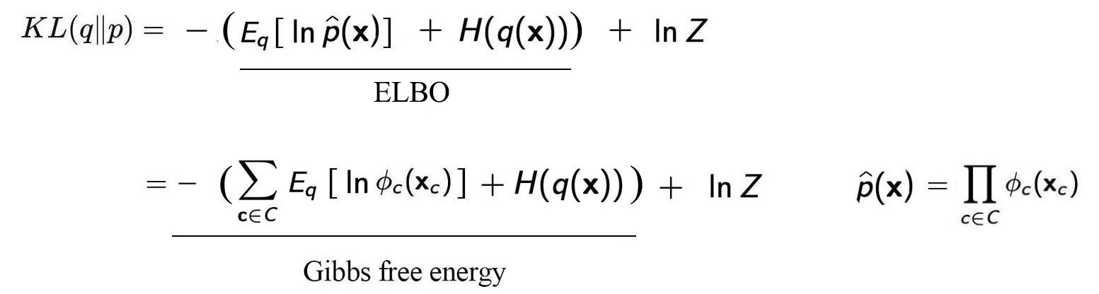
Therefore, minimizing the KL-divergence is equivalent to minimize the Gibbs free energy. We call it free energy because it is the part of the energy that we can manipulate by changing the configuration. This model can be further expanded if we expand the model using an energy model.
Mean Field Variational Inference
(Credit: the proof and the equations are originated from here.)
Don?t get happy too fast. We have missed an important and difficult step in the variational inference. What is the choice of q? It can be extremely hard when q contains multiple variables, i.e. q(z) = q(z?, z?, z?, ?). To further reduce the complexity, the mean field variational inference makes a bold assumption that the distribution can be broken down into distributions each involves one hidden variable only.

Then, we model each distribution with a tractable distribution based on the problem. Our choice of distribution will be easy to analyze analytically. For example, if z? is multinomial, we model it with a multinomial distribution. As mentioned before, many hidden variables depend on each other. So we are going to use coordinate descent to optimize it. We group hidden variables into groups each containing independent variables. We rotate and optimize each group of variables alternatively until the solution converges.
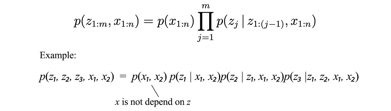
So the last difficult question is how to optimize q?(z?) in each iteration step. We will introduce a few concepts first. The chain rule on probability can be written as the following when x does not depend on z:
Second, since we model q(z) into independent components q?(z?), we can model the entropy as the sum of individual entropy.

With this information, we expand the ELBO

into
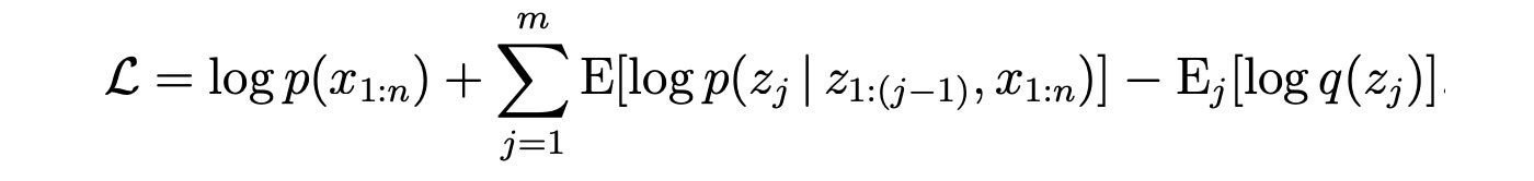
The ordering of z? in z is very arbitrary. In the following equation, we make zk to be the last element. and group everything unrelated to z into a constant. Therefore, the equation becomes

We further remove terms that are unrelated to zk and then express it in the integral form.

We take the derivative and set it to zero to find the optimized distribution q(zk).
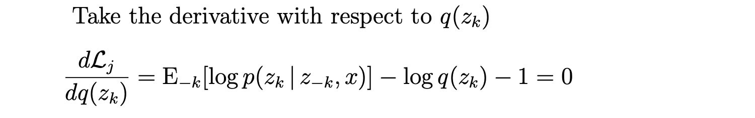
The optimal solution is

with all the constant absorbed and transformed into Z?. We can expand the numerator with Baye?s theorem. Again, the corresponding denominator will be unrelated with zk and therefore absorbed as a normalization factor.

That is the same equation we got in the overview section.

Let?s expand it with q(x) to be q(x?) q(x?) q(x?) ?

This equation can be solved with linear algebra similar to the MAP inference. But we will not detail the solution here.
Recap
We know the equation for the distribution p. But it is nasty to analyze or to manipulate it.

To minimize the difference between p and q, we maximize the ELBO below.

In each iteration step, the optimal solution for the corresponding model parameter z? will be:
Since each q is chosen to be tractable, finding the expectation value or normalization factor (if needed) can be done analytically and pretty straight forward.
Example
(Credit: the example and some equations are originated from here.)
Let?s demonstrate the variation inference with an example. Consider the distribution p(x) below:

where ? (mean) and ? (precision) are modeled by Gaussian and Gamma distribution respectively. So let’s approximate p(x, ?, ?) with q(?, ?). With variance inference, we can learn both parameters from the data. The optimal value for ? and ? in each iteration will satisfy
Therefore, let?s evaluate p(x, ?, ?) by expanding it with the chain rule first and then the definition of p from the problem definition.
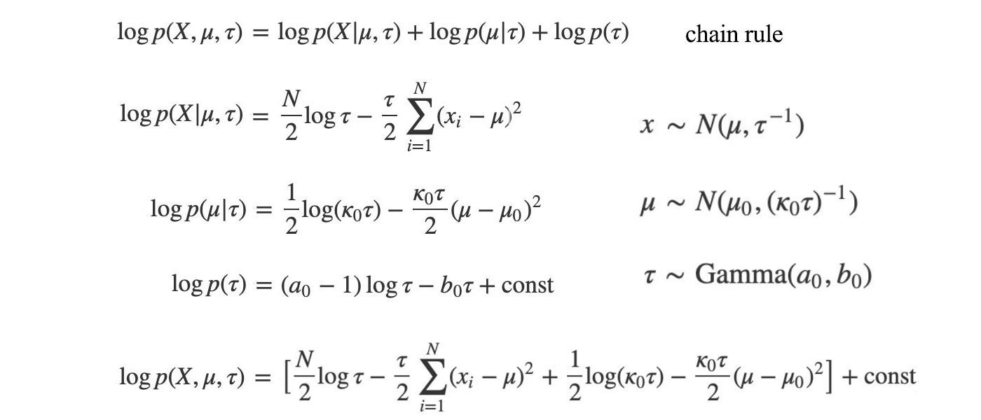
Our next task is to approximate p by q using the mean field variational inference below.

Now, applying the mean field variation inference, we get:
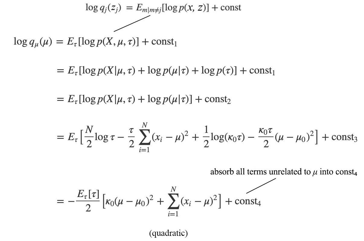
The log q is quadratic. So q is Gaussian distributed.

Our next task is matching the equation above with the Gaussian definition to find the parameter ? and ? (? ? = ?).

Therefore, ? and ? are:
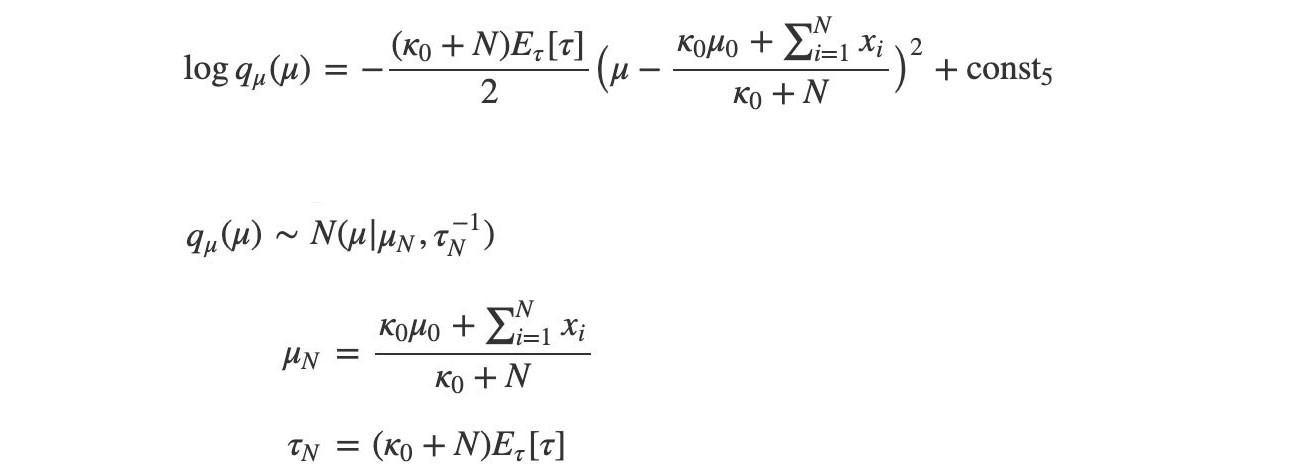
As mentioned, computing the normalization Z is hard in general, but not for these well-known distributions. The normalization factor can be computed by the distribution parameters if needed. We need to focus on finding these parameters instead.
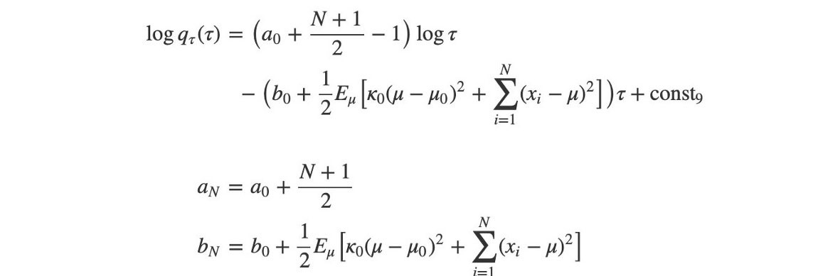
We repeat the same process in computing log q(?).
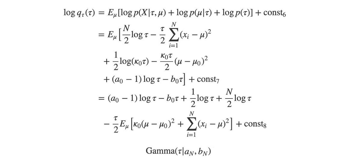
? is Gamma distributed because the distribution above depends on ? and log ? only. The corresponding parameter a and b for the Gamma distribution is:
Now, we have two tractable distributions and we want to find their parameters ? and ?.
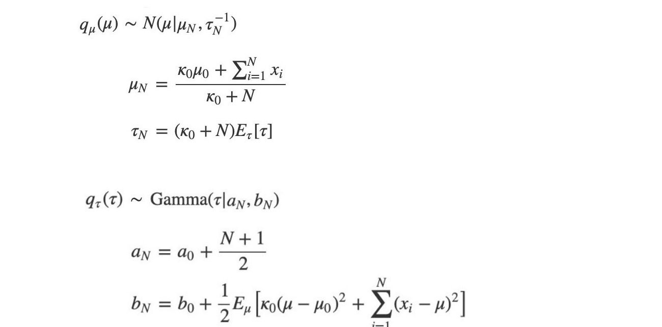
Again, let?s rewrite some terms into expectation forms.
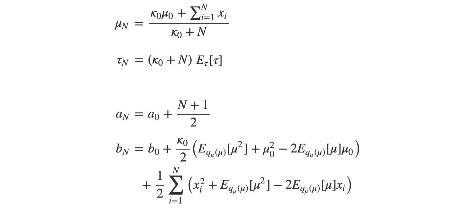
As promised before, mathematical has already solved these expectation terms analytically. We don?t even bother to compute any normalization factor.

? and a can be solved immediately. But ? depend on b, and b depend on ?.

So, we are going to solve them iteratively in alternating steps.
- Initialize ?n to some arbitrary value.
- Solve bn with the equation above.
- Solve ?n with the equation above.
- Repeat the last two steps until the values converge.
Sampling v.s. Variational inference
There is a major shortcoming for sampling methods. We don?t know how far the current sampling solution is from the ground truth. We hope that if we perform enough sampling, the solution is close but there is no quantitative measurement for it. To measure such distance, we need an objective function. Since variational inference is formulated as an optimization problem, we do have certain indications on the progress. However, variational inference approximates the solution rather than finding the exact solution. Indeed, it is unlikely that our solution will be exact.
More readings
Topic modeling is one real-life problem that can be solved with variational inference. For people that want more details:
Machine Learning ? Latent Dirichlet Allocation LDA
Public opinion dominates election results. Unfortunately, with the proliferation of social media, public opinion can be?
medium.com
Credit and references
Probabilistic topic models
Topic models
Latent Dirichlet Allocation
Variational Inference
