Machine Learning — Singular Value Decomposition (SVD) & Principal Component Analysis (PCA)

Photo by Sheldon Nunes

In machine learning (ML), some of the most important linear algebra concepts are the singular value decomposition (SVD) and principal component analysis (PCA). With all the raw data collected, how can we discover structures? For example, with the interest rates of the last 6 days, can we understand its composition to spot trends?

This becomes even harder for high-dimensional raw data. It is like finding a needle in a haystack. SVD allows us to extract and untangle information. In this article, we will detail SVD and PCA. We assume you have basic linear algebra knowledge including rank and eigenvectors. If you experience difficulties in reading this article, I will suggest refreshing those concepts first. At the end of the article, we will answer some questions in the interest rate example above. This article also contains optional sections. Feel free to skip it according to your interest level.

Misconceptions (optional for beginners)

I realize a few common questions that non-beginners may ask. Let me address the elephant in the room first. Is PCA dimension reduction? PCA reduces dimension but it is far more than that. I like the Wiki description (but if you don?t know PCA, this is just gibberish):

Principal component analysis (PCA) is a statistical procedure that uses an orthogonal transformation to convert a set of observations of possibly correlated variables (entities each of which takes on various numerical values) into a set of values of linearly uncorrelated variables called principal components.

From a simplified perspective, PCA transforms data linearly into new properties that are not correlated with each other. For ML, positioning PCA as feature extraction may allow us to explore its potential better than dimension reduction.

What is the difference between SVD and PCA? SVD gives you the whole nine-yard of diagonalizing a matrix into special matrices that are easy to manipulate and to analyze. It lay down the foundation to untangle data into independent components. PCA skips less significant components. Obviously, we can use SVD to find PCA by truncating the less important basis vectors in the original SVD matrix.

Matrix diagonalization

In the article on eigenvalue and eigenvectors, we describe a method to decompose an n n square matrix A into

For example,

However, this is possible only if A is a square matrix and A has n linearly independent eigenvectors. Now, it is time to develop a solution for all matrices using SVD.

Singular vectors & singular values

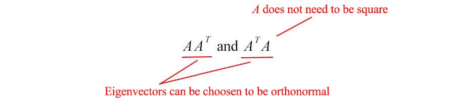
The matrix AA? and A?A are very special in linear algebra. Consider any m n matrix A, we can multiply it with A? to form AA? and A?A separately. These matrices are

• symmetrical,
• square,
• at least positive semidefinite (eigenvalues are zero or positive),
• both matrices have the same positive eigenvalues, and
• both have the same rank r as A.

In addition, the covariance matrices that we often use in ML are in this form. Since they are symmetric, we can choose its eigenvectors to be orthonormal (perpendicular to each other with unit length) ? this is a fundamental property for symmetric matrices.

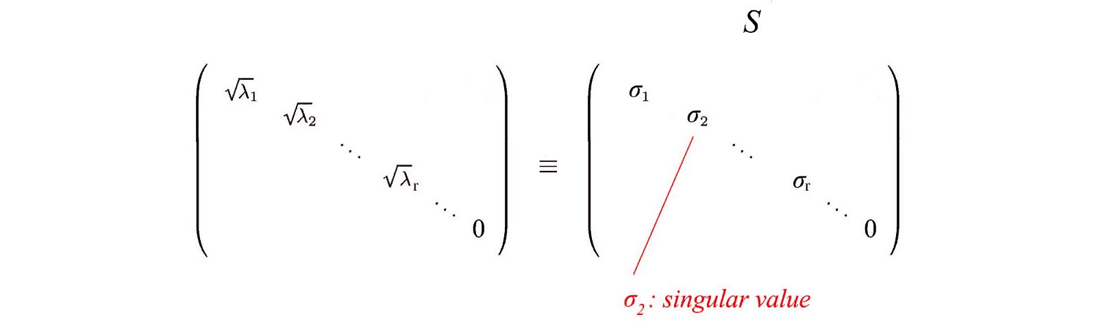
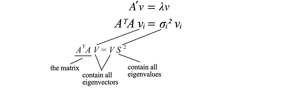
Let?s introduce some terms that frequently used in SVD. We name the eigenvectors for AA? as u? and A?A as v? here and call these sets of eigenvectors u and v the singular vectors of A. Both matrices have the same positive eigenvalues. The square roots of these eigenvalues are called singular values.

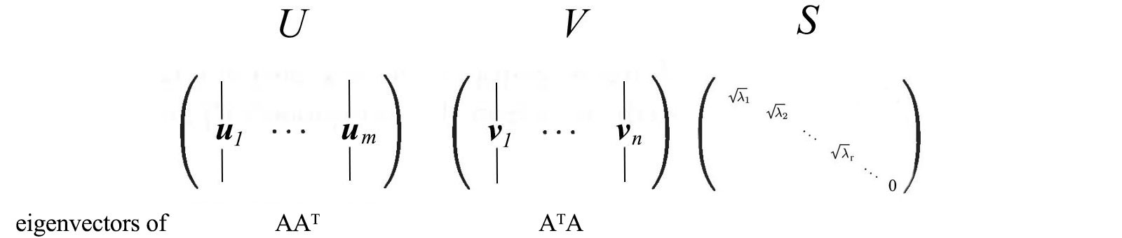
Not too many explanations so far but let?s put everything together first and the explanations will come next. We concatenate vectors u? into U and v? into V to form orthogonal matrices.

Since these vectors are orthonormal, it is easy to prove that U and V obey

SVD

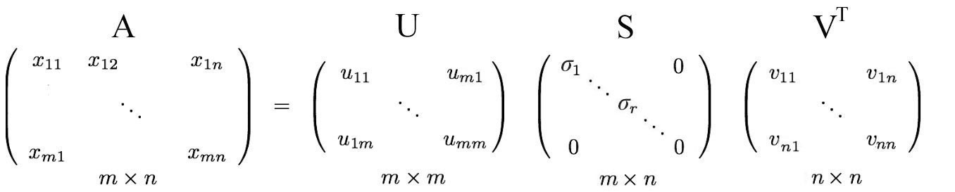
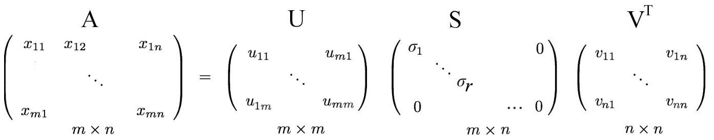
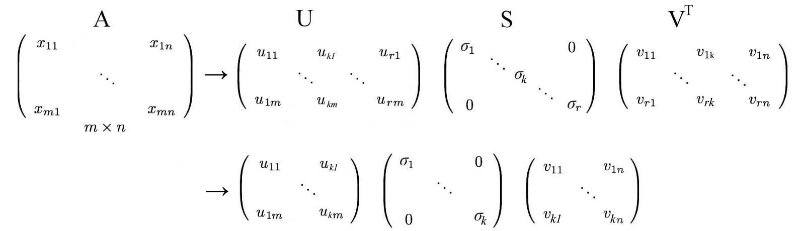
Let?s start with the hard part first. SVD states that any matrix A can be factorized as:

where U and V are orthogonal matrices with orthonormal eigenvectors chosen from AA? and A?A respectively. S is a diagonal matrix with r elements equal to the root of the positive eigenvalues of AA? or A? A (both matrics have the same positive eigenvalues anyway). The diagonal elements are composed of singular values.

i.e. an m n matrix can be factorized as:

We can arrange eigenvectors in different orders to produce U and V. To standardize the solution, we order the eigenvectors such that vectors with higher eigenvalues come before those with smaller values.

Comparing to eigendecomposition, SVD works on non-square matrices. U and V are invertible for any matrix in SVD and they are orthonormal which we love it. Without proof here, we also tell you that singular values are more numerical stable than eigenvalues.

Example (Source of the example)

Before going too far, let?s demonstrate it with a simple example. This will make things very easy to understand.

We calculate:

These matrices are at least positive semidefinite (all eigenvalues are positive or zero). As shown, they share the same positive eigenvalues (25 and 9). The figure below also shows their corresponding eigenvectors.

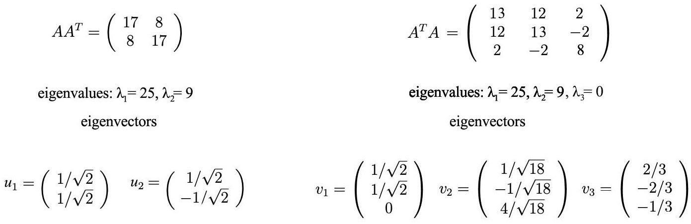
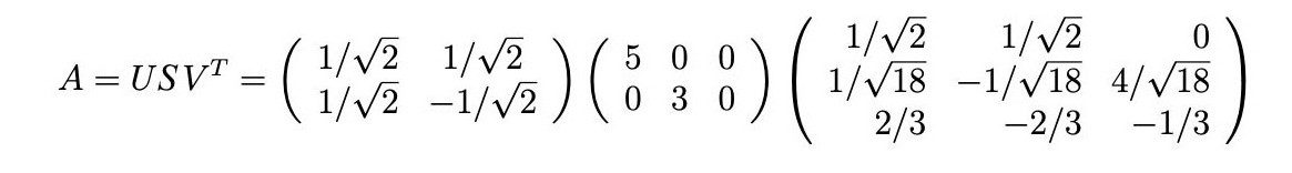
The singular values are the square root of positive eigenvalues, i.e. 5 and 3. Therefore, the SVD composition is

Proof (optional)

To proof SVD, we want to solve U, S, and V with:

We have 3 unknowns. Hopefully, we can solve them with the 3 equations above. The transpose of A is

Knowing

We compute A?A,

The last equation is equilvant to the eigenvector definition for the matrix (A?A). We just put all eigenvectors in a matrix.

with VS equals

V hold all the eigenvectors v? of A?A and S hold the square roots of all eigenvalues of A?A. We can repeat the same process for AA? and come back with a similar equation.

Now, we just solve U, V and S for

and prove the theorem.

Recap

The following is a recap of SVD.

where

Reformulate SVD

Since matrix V is orthogonal, V?V equals I. We can rewrite the SVD equation as:

This equation establishes an important relationship between u? and v?.

Recall

Apply AV = US,

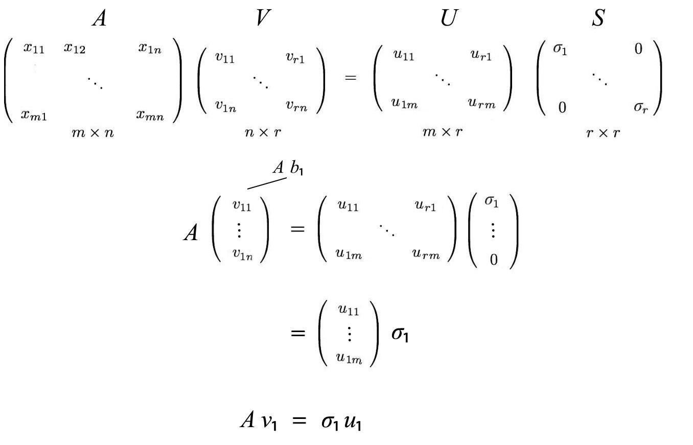
This can be generalized as

Recall,

and

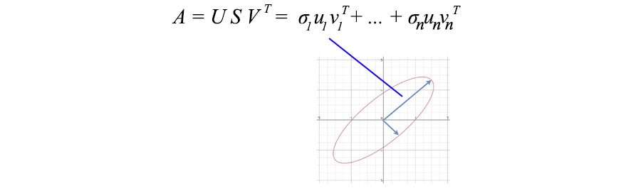
The SVD decomposition can be recognized as a series of outer products of u? and v?.

This formularization of SVD is the key to understand the components of A. It provides an important way to break down an m n array of entangled data into r components. Since u? and v? are unit vectors, we can even ignore terms (??u?v??) with very small singular value ??. (We will come back to this later.)

Let?s first reuse the example before and show how it works.

The matrix A above can be decomposed as

Column space, row space, left nullspace and nullspace (Optional-for advanced users)

Next, we will take a look at what U & V composed of. Let?s say A is an m n matrix of rank r. A?A will be an n n symmetric matrix. All symmetric matrices can choose n orthonormal eigenvectors v?. Because of Av? = ??u? and v? are orthonormal eigenvectors of A?A, we can calculate the value of u??u? as

It equals zero. i.e. u? and u? are orthogonal with each other. As shown previously, they are also eigenvectors of AA?.

From Av? = ?u?, we can recognize that u? is a column vector of A.

Because A has a rank of r, we can choose these r u? vectors to be orthonormal. So what are the remaining m – r orthogonal eigenvectors for AA?? Since left nullspace of A is orthogonal to the column space, it is very natural to pick them as the remaining eigenvector. (The left nullsapce N(A?) is the space span by x in A?x=0.) A similar argument will work for the eigenvectors for A?A. Therefore,

To get back to the former SVD equation from

We simply put back the eigenvectors in the left nullspace and nullspace.

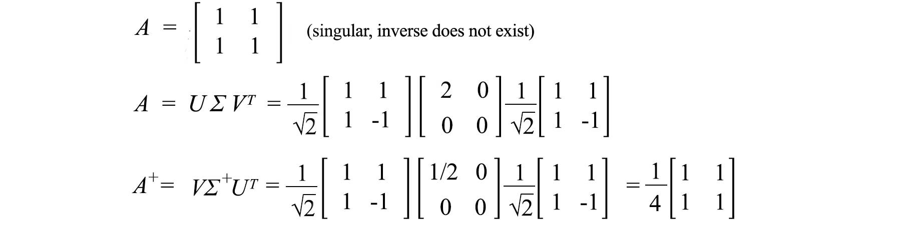
Moore-Penrose Pseudoinverse

For a linear equation system, we can compute the inverse of a square matrix A to solve x.

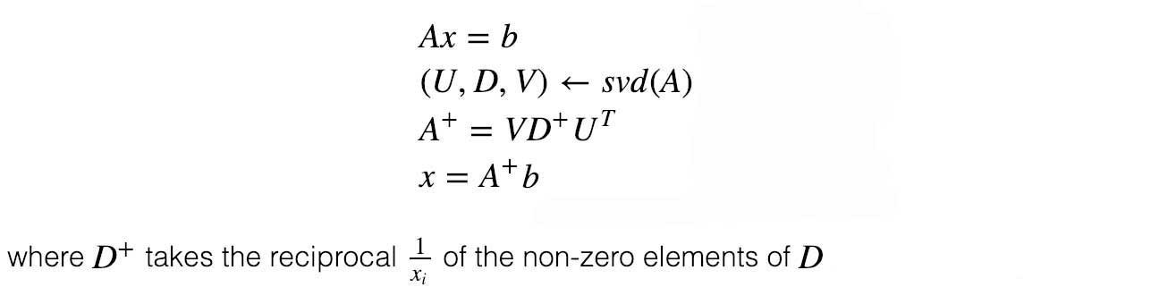
But not all matrices are invertible. Also, in ML, it will be unlikely to find an exact solution with the presence of noise in data. Our objective is to find the model that best fit the data. To find the best-fit solution, we compute a pseudoinverse

which minimizes the least square error below.

And the solution for x can be estimated as,

In a linear regression problem, x is our linear model, A contains the training data and b contains the corresponding labels. We can solve x by

Here is an example.

Variance & covariance

In ML, we identify patterns and relationship. How do we identify the correlation of properties in data? Let?s start the discussion with an example. We sample the height and weight of 12 people and compute their means. We zero-center the original values by subtracting them with its mean. For example, Matrix A below holds the adjusted zero-centered height and weight.

As we plot the data points, we can recognize height and weight are positively related. But how can we quantify such a relationship?

First, how does a property vary? We probably learn the variance from high school. Let?s introduce its cousin. Sample variance is defined as :

Note, it is divided by n-1 instead of n in the variance. With a limited size of the samples, the sample mean is biased and correlated with the samples. The average square distance from this mean will be smaller than that from the general population. The sample covariance S, divided by n-1, compensates for the smaller value and can be proven to be an unbiased estimate for variance ?. (The proof is not very important so I will simply provide a link for the proof here.)

Covariance matrices

Variance measures how a variable varies between itself while covariance is between two variables (a and b).

We can hold all these possible combinations of covariance in a matrix called the covariance matrix ?.

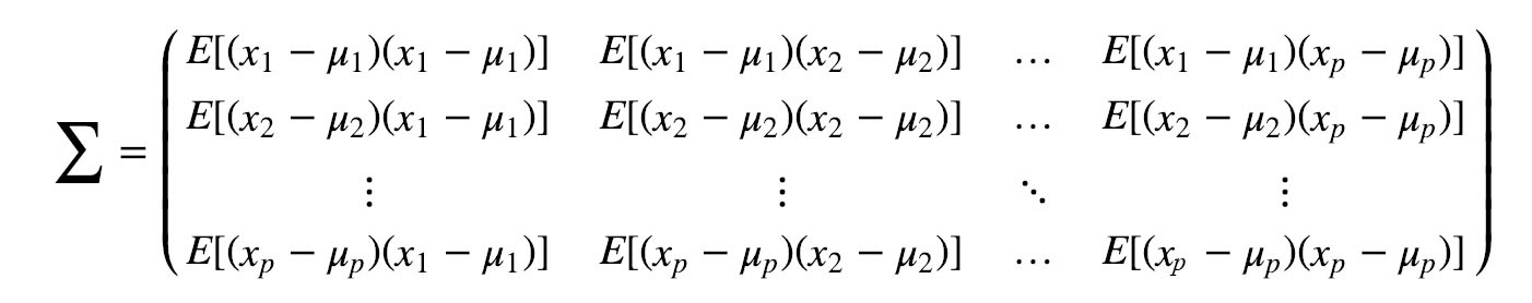
We can rewrite this in a simple matrix form.

The diagonal elements hold the variances of individual variables (like height) and the non-diagonal elements hold the covariance between two variables. Let?s compute the sample covariance now.

The positive sample covariance indicates weight and height are positively correlated. It will be negative if they are negatively correlated and zero if they are independent.

Covariance matrix & SVD

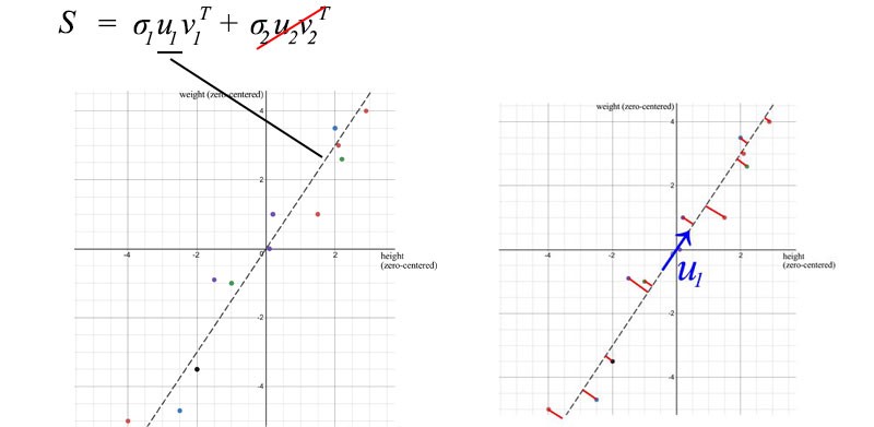
We can use SVD to decompose the sample covariance matrix. Since ?? is relatively small compared with ??, we can even ignore the ?? term. When we train an ML model, we can perform a linear regression on the weight and height to form a new property rather than treating them as two separated and correlated properties (where entangled data usually make model training harder).

u? has one significant importance. It is the principal component of S.

There are a few properties about a sample covariance matrix under the context of SVD:

• The total variance of the data equals the trace of the sample covariance matrix S which equals the sum of squares of S?s singular values. Equipped with this, we can calculate the ratio of variance lost if we drop smaller ?? terms. This reflects the amount of information lost if we eliminate them.

• The first eigenvector u? of S points to the most important direction of the data. In our example, it quantifies the typical ratio between weight and height.

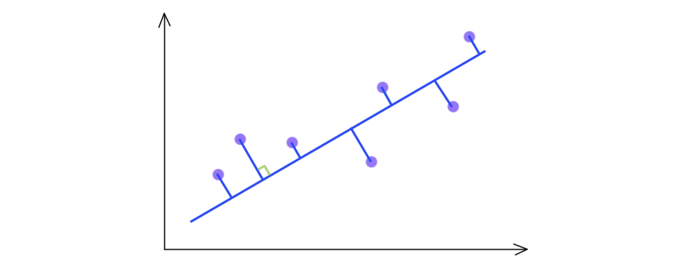
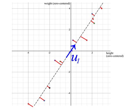Perpendicular least squares

• The error, calculated as the sum of the perpendicular squared distance from the sample points to u?, is the minimum when SVD is used.

Property

Covariance matrices are not only symmetric but they are also positive semidefinite. Because variance is positive or zero, u?Vu below is always greater or equal zero. By the energy test, V is positive semidefinite.

Therefore,

Often, after some linear transformation A, we want to know the covariance of the transformed data. This can be calculated with the transformation matrix A and the covariance of the original data.

Correlation matrix

A correlation matrix is a scaled version of the covariance matrix. A correlation matrix standardizes (scale) the variables to have a standard deviation of 1.

Correlation matrix will be used if variables are in scales of very different magnitudes. Bad scaling may hurt ML algorithms like gradient descent.

Visualization

So far, we have a lot of equations. Let?s visualize what SVD does and develop the insight gradually. SVD factorizes a matrix A into USV?. Applying A to a vector x (Ax) can be visualized as performing a rotation (V?), a scaling (S) and another rotation (U) on x.

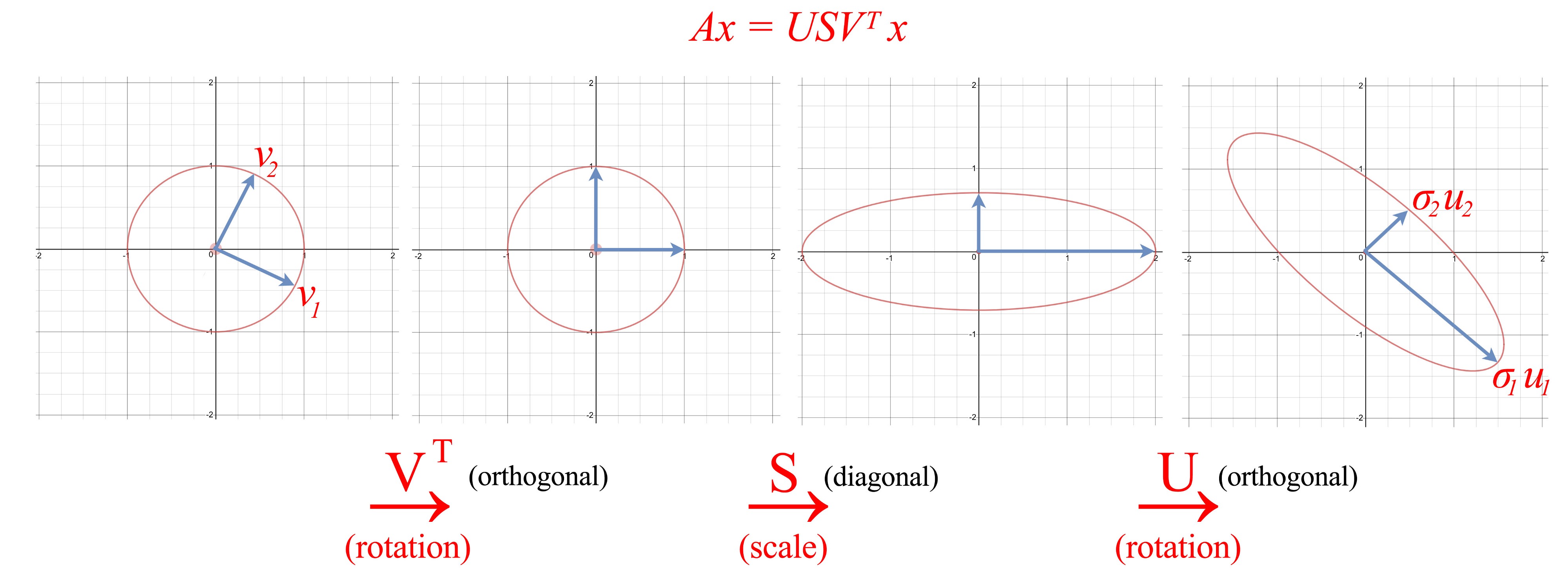
As shown above, the eigenvector v? of V is transformed into:

Or in the full matrix form

demonstrate for r = m < n

Insight of SVD

As described before, the SVD can be formulated as

Since u? and v? have unit length, the most dominant factor in determining the significance of each term is the singular value ??. We purposely sort ?? in the descending order. If the eigenvalues become too small, we can ignore the remaining terms (+ ??u?v?? + ?).

This formularization has some interesting implications. For example, we have a matrix contains the return of stock yields traded by different investors.

As a fund manager, what information can we get out of it? Finding patterns and structures will be the first step. Maybe, we can identify the combination of stocks and investors that have the largest yields. SVD decompose an n n matrix into r components with the singular value ?? demonstrating its significant. Consider this as a way to extract entangled and related properties into fewer principal directions with no correlations.

If data is highly correlated, we should expect many ?? values to be small and can be ignored.

In our previous example, weight and height are highly related. If we have a matrix containing the weight and height of 1000 people, the first component in the SVD decomposition will dominate. The u? vector indeed demonstrates the ratio between weight and height among these 1000 people as we discussed before.

Principal Component Analysis (PCA)

Technically, SVD extracts data in the directions with the highest variances respectively. PCA is a linear model in mapping m-dimensional input features to k-dimensional latent factors (k principal components). If we ignore the less significant terms, we remove the components that we care less but keep the principal directions with the highest variances (largest information).

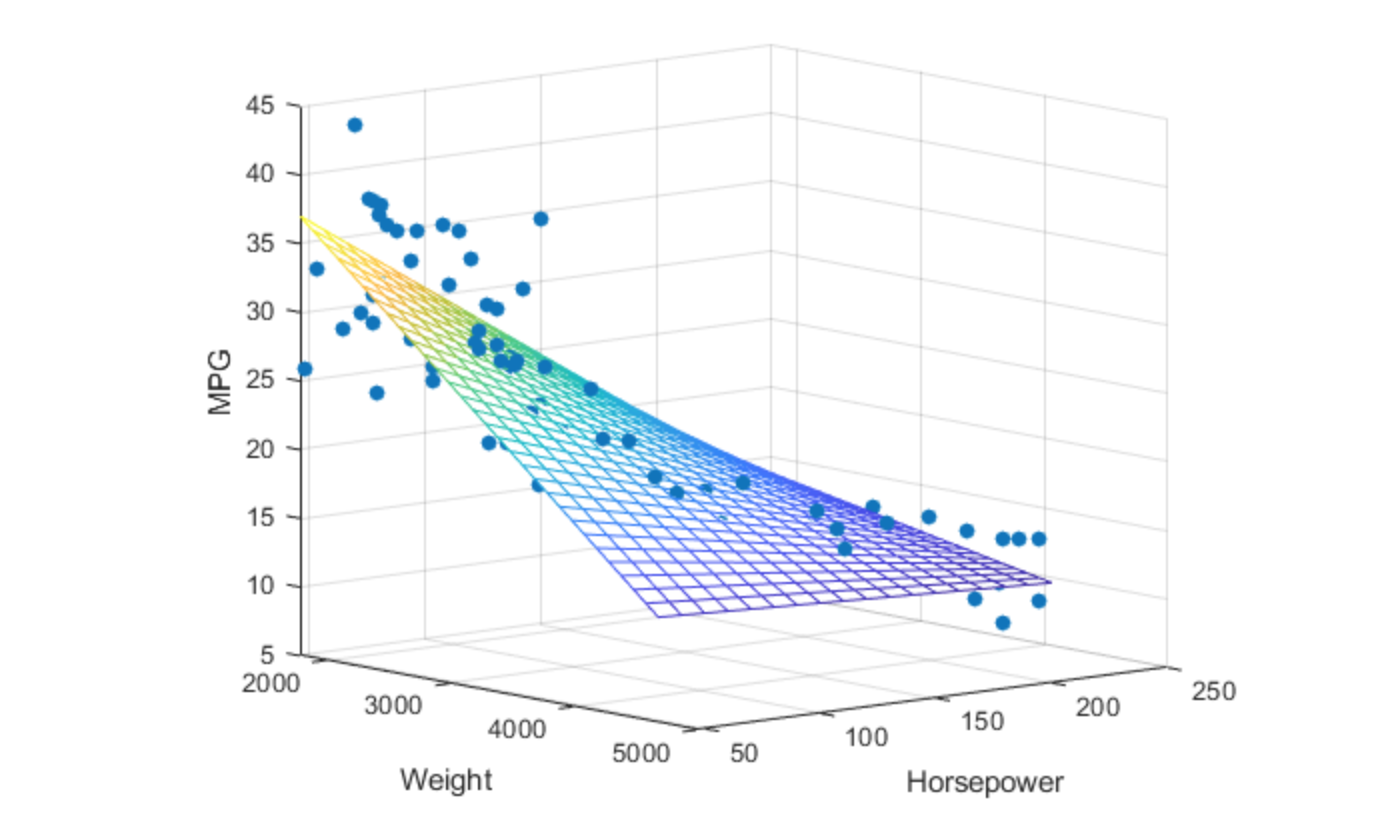
Consider the 3-dimensional data points that displayed as blue dots below. It can be approximated by a plane easily.

Source

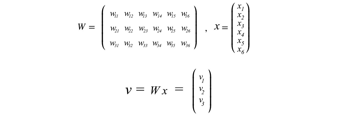
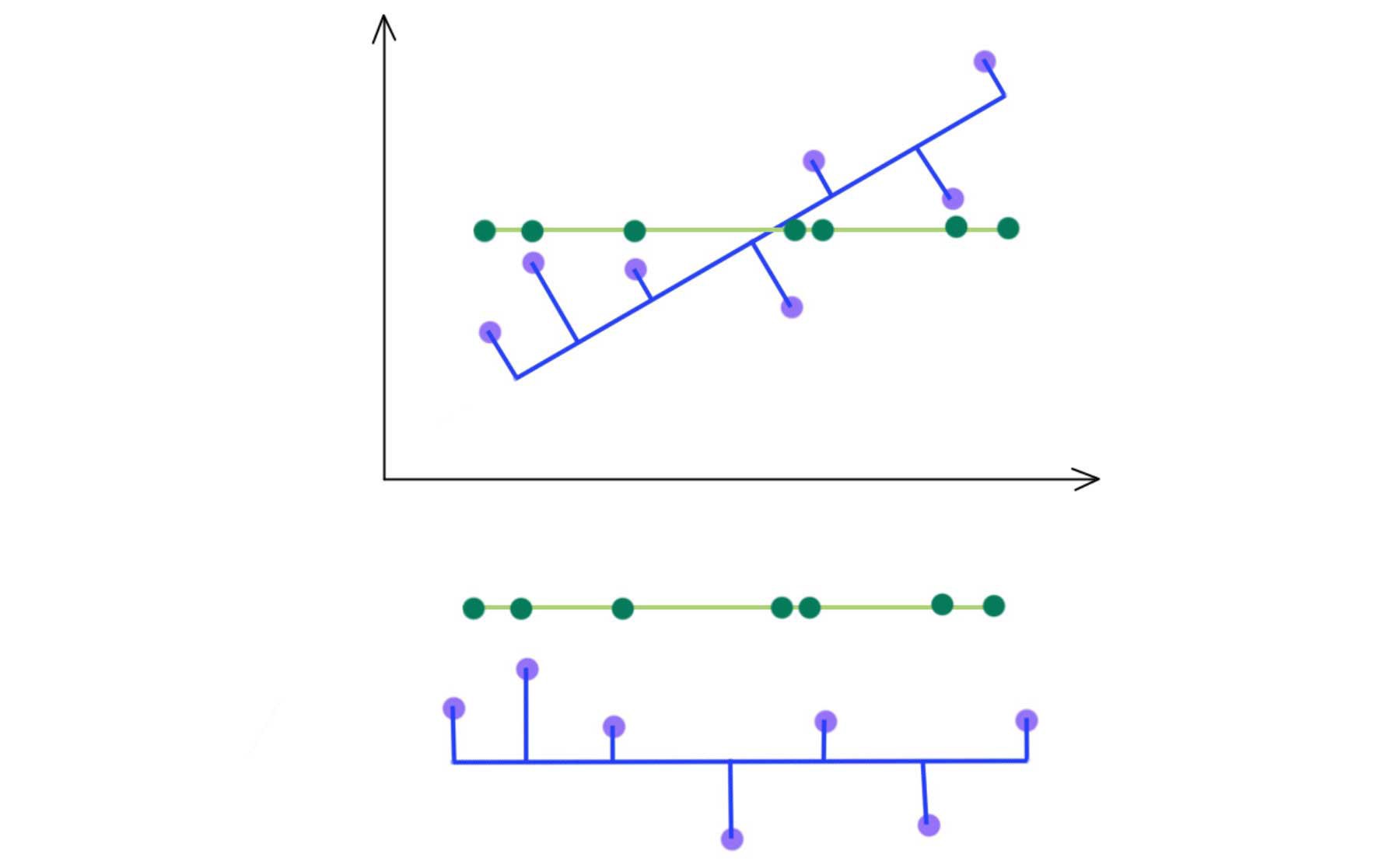
You may quickly realize that we can use SVD to find the matrix W. Consider the data points below that lie on a 2-D space.

SVD selects a projection that maximizes the variance of their output. Hence, PCA will pick the blue line over the green line if it has a higher variance.

As indicated below, we keep the eigenvectors that have the top kth highest singular value.

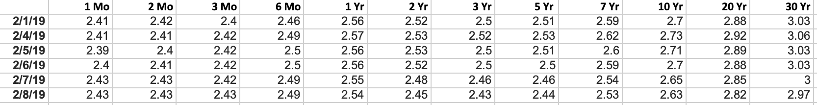
Interest rate

Let?s illustrate the concept deeper by retracing an example here with the interest rate data originated from the US Treasurer Department. The basis points for 9 different interest rates (from 3 months, 6 months, ? to 20 years) over 6 consecutive business days are collected with A stored the difference from the previous date. A also has its elements subtracted by its mean over this period already. i.e. it is zero-centered (across its row).

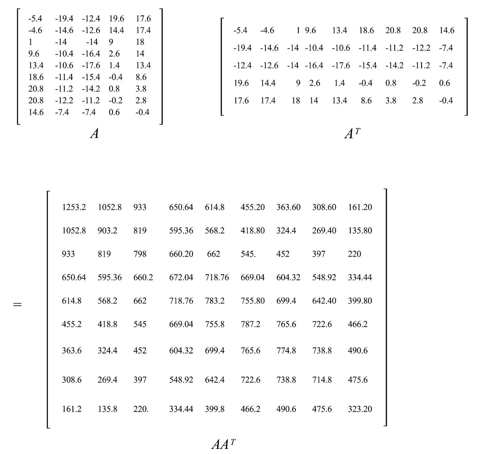
The sample covariance matrix equals S = AA?/(5?1).

Now we have the covariance matrix S that we want to factorize. The SVD decomposition is

From the SVD decomposition, we realize that we can focus on the first three principal components.

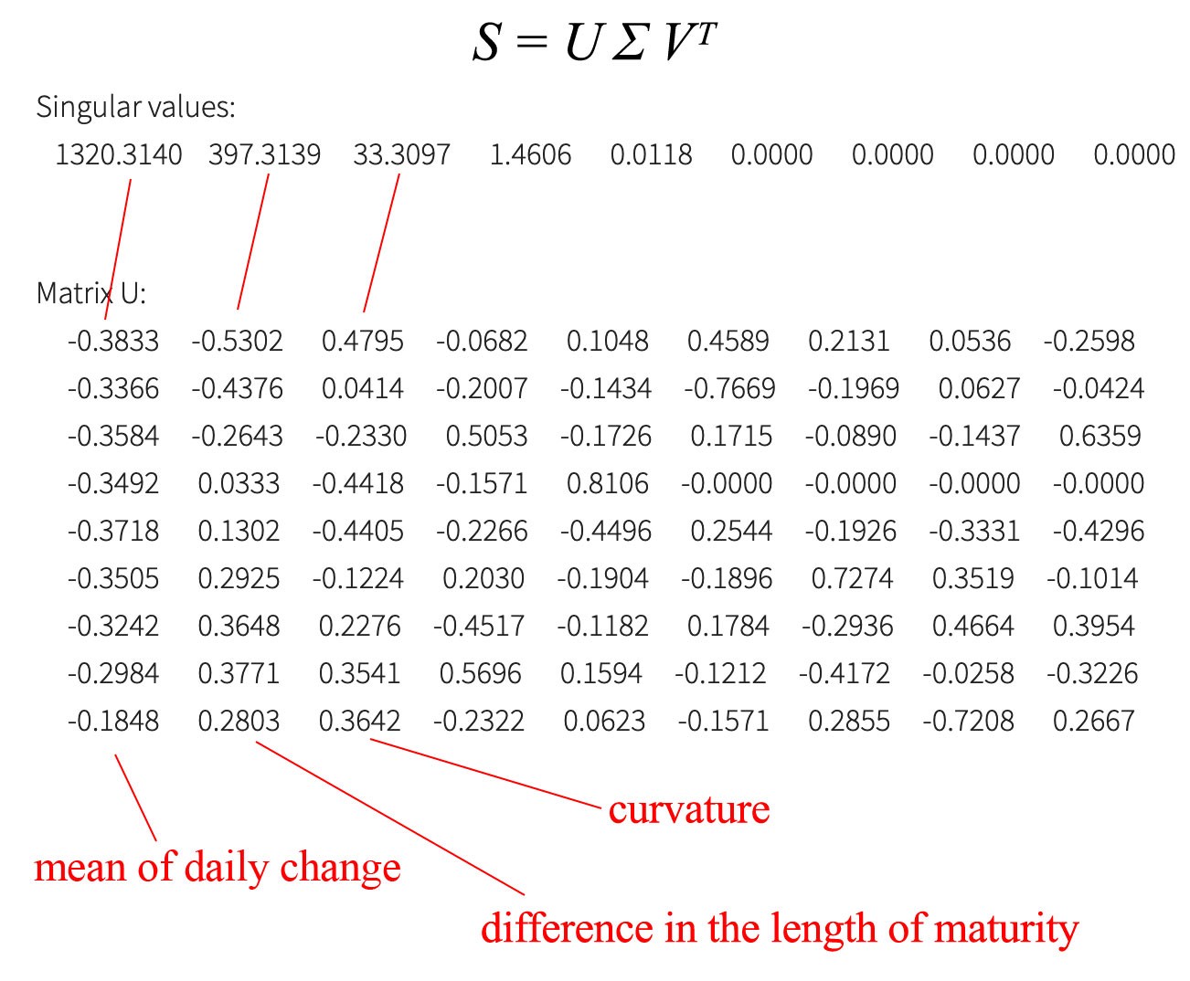
As shown, the first principal component is related to a weighted average of the daily change for all maturity lengths. The second principal component adjusts the daily change sensitive to the maturity length of the bond. (The third principal component is likely the curvature ? a second-degree derivative.)

We understand the relationship between the interesting rate change and maturity well in our daily life. So the principal components reconfirm what we believe how interest rates behave. But when we are presented with unfamiliar raw data, PCA is very helpful to extract the principal components of your data to find the underneath information structure. This may answer some questions on how to find a needle in a haystack.

Tips

Scale features before performing SVD.

Say, we want to retain 99% variance, we can choose k such that