Simplifying a complex algorithm
Motivation
Although most of the Kaggle competition winners use stack/ensemble of various models, one particular model that is part of most of the ensembles is some variant of Gradient Boosting (GBM) algorithm. Take for an example the winner of latest Kaggle competition: Michael Jahrer?s solution with representation learning in Safe Driver Prediction. His solution was a blend of 6 models. 1 LightGBM (a variant of GBM) and 5 Neural Nets. Although his success is attributed to the semi-supervised learning that he used for the structured data, but gradient boosting model has done the useful part too.
Even though GBM is being used widely, many practitioners still treat it as complex black-box algorithm and just run the models using pre-built libraries. The purpose of this post is to simplify a supposedly complex algorithm and to help the reader to understand the algorithm intuitively. I am going to explain the pure vanilla version of the gradient boosting algorithm and will share links for its different variants at the end. I have taken base DecisionTree code from fast.ai library (fastai/courses/ml1/lesson3-rf_foundations.ipynb) and on top of that, I have built my own simple version of basic gradient boosting model.
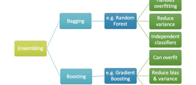
Brief description for Ensemble, Bagging and Boosting
When we try to predict the target variable using any machine learning technique, the main causes of difference in actual and predicted values are noise, variance, and bias. Ensemble helps to reduce these factors (except noise, which is irreducible error)
An ensemble is just a collection of predictors which come together (e.g. mean of all predictions) to give a final prediction. The reason we use ensembles is that many different predictors trying to predict same target variable will perform a better job than any single predictor alone. Ensembling techniques are further classified into Bagging and Boosting.
- Bagging is a simple ensembling technique in which we build many independent predictors/models/learners and combine them using some model averaging techniques. (e.g. weighted average, majority vote or normal average)
We typically take random sub-sample/bootstrap of data for each model, so that all the models are little different from each other. Each observation is chosen with replacement to be used as input for each of the model. So, each model will have different observations based on the bootstrap process. Because this technique takes many uncorrelated learners to make a final model, it reduces error by reducing variance. Example of bagging ensemble is Random Forest models.
- Boosting is an ensemble technique in which the predictors are not made independently, but sequentially.
This technique employs the logic in which the subsequent predictors learn from the mistakes of the previous predictors. Therefore, the observations have an unequal probability of appearing in subsequent models and ones with the highest error appear most. (So the observations are not chosen based on the bootstrap process, but based on the error). The predictors can be chosen from a range of models like decision trees, regressors, classifiers etc. Because new predictors are learning from mistakes committed by previous predictors, it takes less time/iterations to reach close to actual predictions. But we have to choose the stopping criteria carefully or it could lead to overfitting on training data. Gradient Boosting is an example of boosting algorithm.
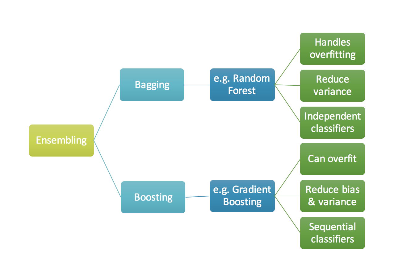 Fig 1. Ensembling
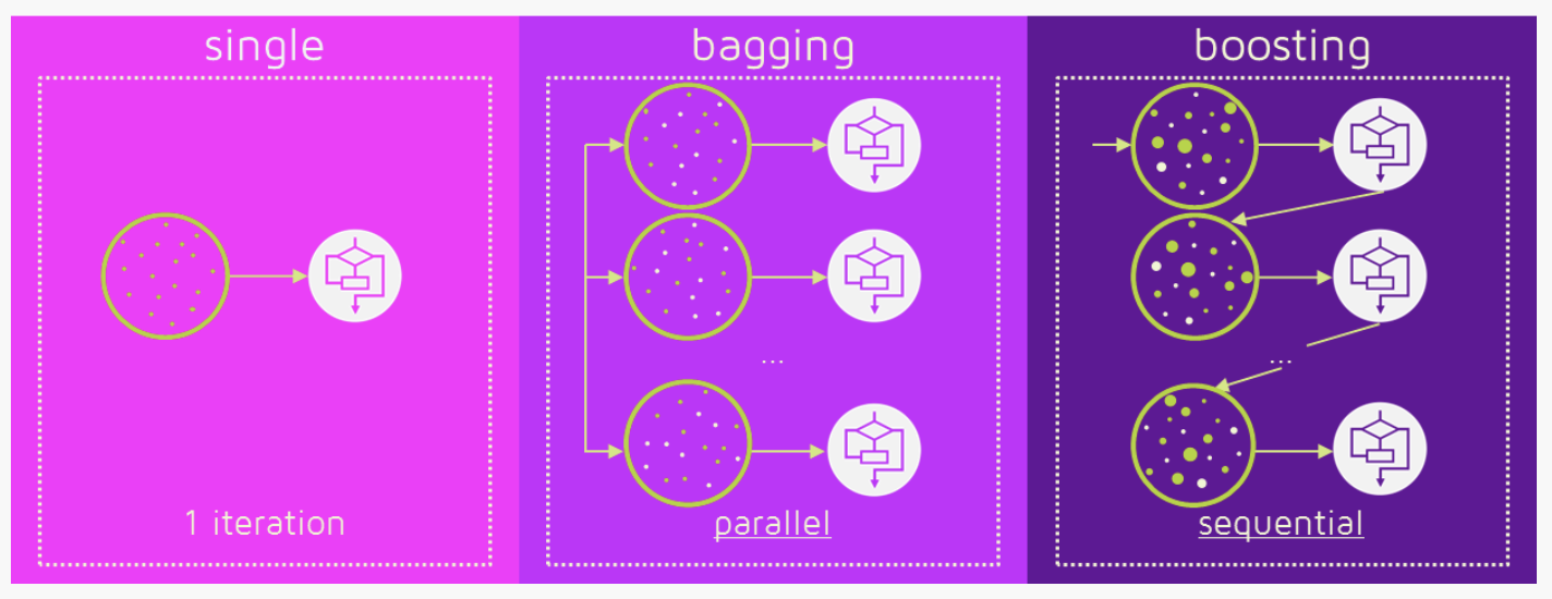 Fig 2. Bagging (independent models) & Boosting (sequential models). Reference: https://quantdare.com/what-is-the-difference-between-bagging-and-boosting/
Gradient Boosting algorithm
Gradient boosting is a machine learning technique for regression and classification problems, which produces a prediction model in the form of an ensemble of weak prediction models, typically decision trees. (Wikipedia definition)
The objective of any supervised learning algorithm is to define a loss function and minimize it. Let?s see how maths work out for Gradient Boosting algorithm. Say we have mean squared error (MSE) as loss defined as:
We want our predictions, such that our loss function (MSE) is minimum. By using gradient descent and updating our predictions based on a learning rate, we can find the values where MSE is minimum.
So, we are basically updating the predictions such that the sum of our residuals is close to 0 (or minimum) and predicted values are sufficiently close to actual values.
Intuition behind Gradient Boosting
The logic behind gradient boosting is simple, (can be understood intuitively, without using mathematical notation). I expect that whoever is reading this post might be familiar with simple linear regression modeling.
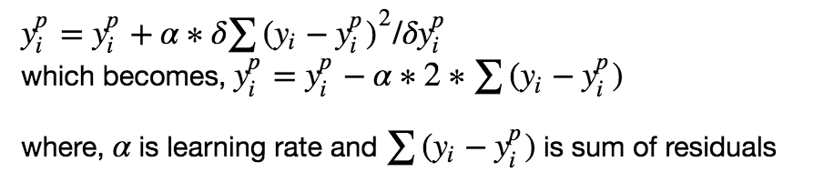
A basic assumption of linear regression is that sum of its residuals is 0, i.e. the residuals should be spread randomly around zero.
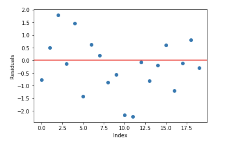 Fig 3. Sample random normally distributed residuals with mean around 0
Now think of these residuals as mistakes committed by our predictor model. Although, tree-based models (considering decision tree as base models for our gradient boosting here) are not based on such assumptions, but if we think logically (not statistically) about this assumption, we might argue that, if we are able to see some pattern of residuals around 0, we can leverage that pattern to fit a model.
So, the intuition behind gradient boosting algorithm is to repetitively leverage the patterns in residuals and strengthen a model with weak predictions and make it better. Once we reach a stage that residuals do not have any pattern that could be modeled, we can stop modeling residuals (otherwise it might lead to overfitting). Algorithmically, we are minimizing our loss function, such that test loss reach its minima.
In summary, ? We first model data with simple models and analyze data for errors. ? These errors signify data points that are difficult to fit by a simple model. ? Then for later models, we particularly focus on those hard to fit data to get them right. ? In the end, we combine all the predictors by giving some weights to each predictor.
A more technical quotation of the same logic is written in Probably Approximately Correct: Nature?s Algorithms for Learning and Prospering in a Complex World,
?The idea is to use the weak learning method several times to get a succession of hypotheses, each one refocused on the examples that the previous ones found difficult and misclassified. ? Note, however, it is not obvious at all how this can be done?
Steps to fit a Gradient Boosting model
Let?s consider simulated data as shown in scatter plot below with 1 input (x) and 1 output (y) variables.
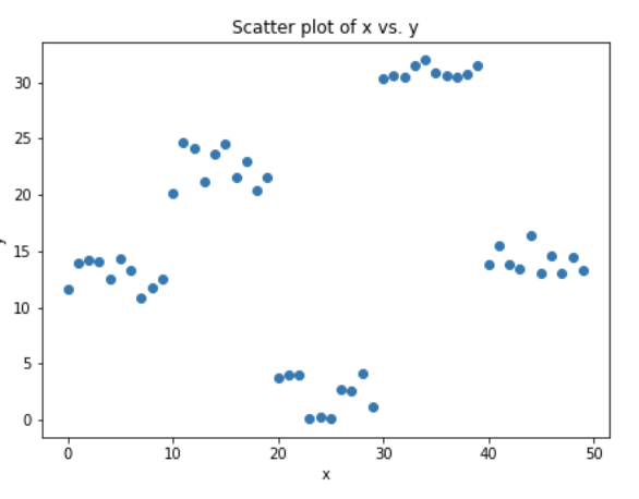 Fig 4. Simulated data (x: input, y: output)
Data for above shown plot is generated using below python code:
Code Chunk 1. Data simulation
1. Fit a simple linear regressor or decision tree on data (I have chosen decision tree in my code) [call x as input and y as output]
Code Chunk 2. (Step 1)Using decision tree to find best split (here depth of our tree is 1)
2. Calculate error residuals. Actual target value, minus predicted target value [e1= y – y_predicted1 ]
3. Fit a new model on error residuals as target variable with same input variables [call it e1_predicted]
4. Add the predicted residuals to the previous predictions[y_predicted2 = y_predicted1 + e1_predicted]
5. Fit another model on residuals that is still left. i.e. [e2 = y – y_predicted2] and repeat steps 2 to 5 until it starts overfitting or the sum of residuals become constant. Overfitting can be controlled by consistently checking accuracy on validation data.
Code Chunk 3. (Steps 2 to 5) Calculate residuals and update new target variable and new predictions
To aid the understanding of the underlying concepts, here is the link with complete implementation of a simple gradient boosting model from scratch. [Link: Gradient Boosting from scratch]
Shared code is a non-optimized vanilla implementation of gradient boosting. Most of the gradient boosting models available in libraries are well optimized and have many hyper-parameters.
Visualization of working Gradient Boosting Tree
Blue dots (left) plots are input (x) vs. output (y) ? Red line (left) shows values predicted by decision tree ? Green dots (right) shows residuals vs. input (x) for ith iteration ? Iteration represent sequential order of fitting gradient boosting tree
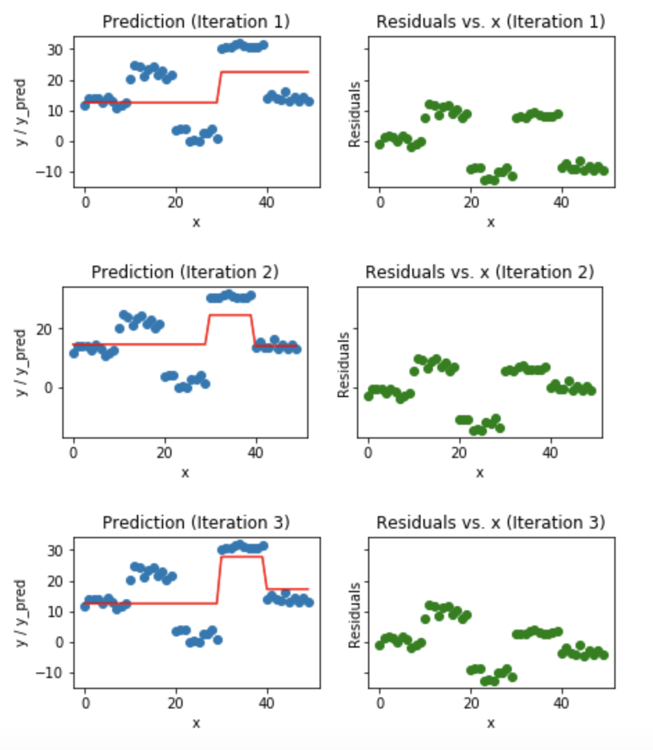 Fig 5. Visualization of gradient boosting predictions (First 4 iterations)
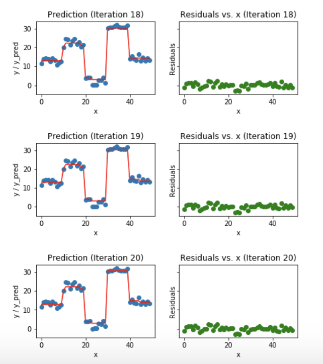 Fig 6. Visualization of gradient boosting predictions (18th to 20th iterations)
We observe that after 20th iteration , residuals are randomly distributed (I am not saying random normal here) around 0 and our predictions are very close to true values. (iterations are called n_estimators in sklearn implementation). This would be a good point to stop or our model will start overfitting.
Let?s see how our model look like for 50th iteration.
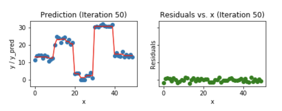 Fig 7. Visualization of gradient boosting prediction (iteration 50th)
We see that even after 50th iteration, residuals vs. x plot look similar to what we see at 20th iteration. But the model is becoming more complex and predictions are overfitting on the training data and are trying to learn each training data. So, it would have been better to stop at 20th iteration.
Python code snippet used for plotting all the above figures.
Code Chunk 4. Plotting predictions and residuals (fed in 1st code chunk?s loop)
I hope that this blog helped you to get basic intuition behind how gradient boosting works. To understand gradient boosting for regression in detail, I would strongly recommend you to read this amazing article by the faculty at University of San Francisco, Terence Parr (Creator of the ANTLR parser generator) and Jeremy Howard (Founding researcher at fast.ai) : How to explain gradient boosting.
More useful resources
- My github repo and kaggle kernel link for GBM from scratch:https://www.kaggle.com/grroverpr/gradient-boosting-simplified/https://nbviewer.jupyter.org/github/groverpr/Machine-Learning/blob/master/notebooks/01_Gradient_Boosting_Scratch.ipynb
- A detailed and intuitive explanation of gradient boosting: How to explain gradient boosting by Terence Parr and Jeremy Howard
- Fast.ai github repo link for DecisionTree from scratch (Massive ML/DL related resources): https://github.com/fastai/fastai
- Video by Alexander Ihler. This video really helped me to build my understanding.
4. A Kaggle Master Explains Gradient Boosting: Ben Gorman
A Kaggle Master Explains Gradient Boosting
If linear regression was a Toyota Camry, then gradient boosting would be a UH-60 Blackhawk Helicopter. A particular?
blog.kaggle.com
5. Widely used GBM algorithms: XGBoost || Lightgbm || Catboost || sklearn.ensemble.GradientBoostingClassifier

