
In previous two articles, we introduced reinforcement learning definition, examples, and simple solving strategies using random policy search and genetic algorithms.
In practice, random search does not work well for complex problems where the search space (that depends on the number of possible states and actions) is large. Also, genetic algorithm is a meta-heuristic optimization so it does not provide a guarantee to find an optimal solution. In this article, we are going to introduce fundamental reinforcement learning algorithms.
We start by reviewing the Markov Decision Process formulation, then we describe the value-iteration and policy iteration which are algorithms for finding the optimal policy when the agent knows sufficient details about the environment model. We then, describe the Q-learning is a model-free learning that can be used when the agent does not know the environment model but has to discover the policy by trial and error making use of its history of interaction with the environment. We also provide demonstration examples of the three methods by using the FrozenLake8x8 and MountainCar problems from OpenAI gym.
Markov Decision Process (MDP)
We briefly introduced Markov Decision Process MDPin our first article. To recall, in reinforcement learning problems we have an agent interacting with an environment. At each time step, the agent performs an action which leads to two things: changing the environment state and the agent (possibly) receiving a reward (or penalty) from the environment. The goal of the agent is to discover an optimal policy (i.e. what actions to do in each state) such that it maximizes the total value of rewards received from the environment in response to its actions. MDPis used to describe the agent/ environment interaction settings in a formal way.
MDP consists of a tuple of 5 elements:
- S : Set of states. At each time step the state of the environment is an element s ? S.
- A: Set of actions. At each time step the agent choses an action a ? A to perform.
- p(s_{t+1} | s_t, a_t) : State transition model that describes how the environment state changes when the user performs an action a depending on the action aand the current state s.
- p(r_{t+1} | s_t, a_t) : Reward model that describes the real-valued reward value that the agent receives from the environment after performing an action. In MDP the the reward value depends on the current state and the action performed.
- ? : discount factor that controls the importance of future rewards. We will describe it in more details later.
The way by which the agent chooses which action to perform is named the agent policy which is a function that takes the current environment state to return an action. The policy is often denoted by the symbol ?.

Let?s now differentiate between two types environments.
Deterministic environment: deterministic environment means that both state transition model and reward model are deterministic functions. If the agent while in a given state repeats a given action, it will always go the same next state and receive the same reward value.
Stochastic environment: In a stochastic environment there is uncertainty about the actions effect. When the agent repeats doing the same action in a given state, the new state and received reward may not be the same each time. For example, a robot which tries to move forward but because of the imperfection in the robot operation or other factors in the environment (e.g. slippery floor), sometimes the action forward will make it move forward but in sometimes, it will move to left or right.
Deterministic environments are easier to solve, because the agent knows how to plan its actions with no-uncertainty given the environment MDP. Possibly, the environment can be modeled in as a graph where each state is a node and edges represent transition actions from one state to another and edge weights are received rewards. Then, the agent can use a graph search algorithm such as A* to find the path with maximum total reward form the initial state.
Total reward
Remember, that the goal of the agent is to pick the best policy that will maximize the total rewards received from the environment.
Assume that environment is initially at state s_0
At time 0 : Agent observes the environment state s_0 and picks an action a_0, then upon performing its action, environment state becomes s_1 and the agent receives a reward r_1 .
At time 1: Agent observes current state s_1 and picks an action a_1 , then upon acting its action, environment state becomes s_2 and it receives a reward r_2 .
At time 2: Agent observes current state s_2 and picks an action a_2 , then upon acting its action, environment state becomes s_3 and it receives a reward r_3 .
So the total reward received by the agent in response to the actions selected by its policy is going to be:
Total reward = r_1 + r_2 + r_3 + r_4 + r_5 + ..
However, it is common to use a discount factor to give higher weight to near rewards received near than rewards received further in the future.
Total discounted reward = r_1 + ? r_2 + ? r_3 + ? r_4 + ?? r_5+ ?so,

where T is the horizon (episode length) which can be infinity if there is maximum length for the episode.
The reason for using discount factor is to prevent the total reward from going to infinity (because 0 ? ? ? 1), it also models the agent behavior when the agent prefers immediate rewards than rewards that are potentially received far away in the future. (If I give you 1000 dollars today and If I give you 1000 days after 10 years which one would you prefer ? ). Imagine a robot that is trying to solve a maze and there are two paths to the goal state one of them is longer but gives higher reward while there is a shorter path with smaller reward. By adjusting the ? value, you can control which the path the agent should prefer.
Now, we are ready to introduce the value-iteration and policy-iteration algorithms. These are two fundamental methods for solving MDPs. Both value-iteration and policy-iteration assume that the agent knows the MDP model of the world (i.e. the agent knows the state-transition and reward probability functions). Therefore, they can be used by the agent to (offline) plan its actions given knowledge about the environment before interacting with it. Later, we will discuss Q-learning which is a model-free learning environment that can be used in situation where the agent initially knows only that are the possible states and actions but doesn’t know the state-transition and reward probability functions. In Q-learning the agent improves its behavior (online) through learning from the history of interactions with the environment.
Value function
Many reinforcement learning introduce the notion of `value-function` which often denoted as V(s) . The value function represent how good is a state for an agent to be in. It is equal to expected total reward for an agent starting from state s. The value function depends on the policy by which the agent picks actions to perform. So, if the agent uses a given policy ? to select actions, the corresponding value function is given by:

Among all possible value-functions, there exist an optimal value function that has higher value than other functions for all states.

The optimal policy ?* is the policy that corresponds to optimal value function.

In addition to the state value-function, for convenience RL algorithms introduce another function which is the state-action pair Q function. Q is a function of a state-action pair and returns a real value.

The optimal Q-function Q*(s, a) means the expected total reward received by an agent starting in sand picks action a, then will behave optimally afterwards. There, Q*(s, a) is an indication for how good it is for an agent to pick action a while being in state s.
Since V*(s) is the maximum expected total reward when starting from state s , it will be the maximum of Q*(s, a)over all possible actions.
Therefore, the relationship between Q*(s, a) and V*(s) is easily obtained as:

and If we know the optimal Q-function Q*(s, a) , the optimal policy can be easily extracted by choosing the action a that gives maximum Q*(s, a) for state s.

Now, lets introduce an important equation called the Bellman equation which is a super-important equation optimization and have applications in many fields such as reinforcement learning, economics and control theory. Bellman equation using dynamic programming paradigm provides a recursive definition for the optimal Q-function.The Q*(s, a) is equal to the summation of immediate reward after performing action a while in state s and the discounted expected future reward after transition to a next state s’.

Value-iteration and policy iteration rely on these equations to compute the optimal value-function.
Value Iteration
Value iteration computes the optimal state value function by iteratively improving the estimate of V(s). The algorithm initialize V(s) to arbitrary random values. It repeatedly updates the Q(s, a) and V(s) values until they converges. Value iteration is guaranteed to converge to the optimal values. This algorithm is shown in the following pseudo-code:
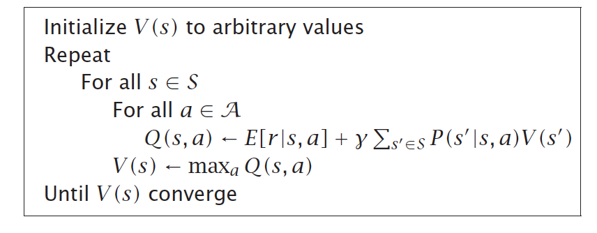 Pseudo code for value-iteration algorithm. Credit: Alpaydin Introduction to Machine Learning, 3rd edition.
Example : FrozenLake8x8 (Using Value-Iteration)
Now lets implement it in python to solve the FrozenLake8x8 openAI gym. compared to the FrozenLake-v0 environment we solved earlier using genetic algorithm, the FrozenLake8x8 has 64 possible states (grid size is 8×8) instead of 16. Therefore, the problem becomes harder and genetic algorithm will struggle to find the optimal solution.
Solution of the FrozenLake8x8 environment using Value-Iteration
Policy Iteration
While value-iteration algorithm keeps improving the value function at each iteration until the value-function converges. Since the agent only cares about the finding the optimal policy, sometimes the optimal policy will converge before the value function. Therefore, another algorithm called policy-iteration instead of repeated improving the value-function estimate, it will re-define the policy at each step and compute the value according to this new policy until the policy converges. Policy iteration is also guaranteed to converge to the optimal policy and it often takes less iterations to converge than the value-iteration algorithm.
The pseudo code for Policy Iteration is shown below.
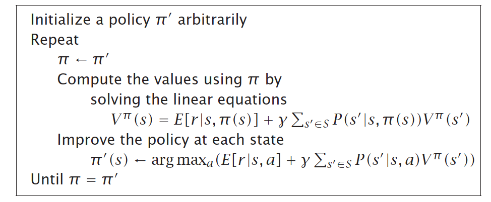 Pseudo code for policy-iteration algorithm. Credit: Alpaydin Introduction to Machine Learning, 3rd edition.
Example : FrozenLake8x8 (Using Policy-Iteration)
Solution of the FrozenLake8x8 environment using Policy Iteration
Value-Iteration vs Policy-Iteration
Both value-iteration and policy-iteration algorithms can be used for offline planning where the agent is assumed to have prior knowledge about the effects of its actions on the environment (they assume the MDP model is known). Comparing to each other, policy-iteration is computationally efficient as it often takes considerably fewer number of iterations to converge although each iteration is more computationally expensive.
Q-Learning
Now, lets consider the case where the agent does not know apriori what are the effects of its actions on the environment (state transition and reward models are not known). The agent only knows what are the set of possible states and actions, and can observe the environment current state. In this case, the agent has to actively learn through the experience of interactions with the environment. There are two categories of learning algorithms:
model-based learning: In model-based learning, the agent will interact to the environment and from the history of its interactions, the agent will try to approximate the environment state transition and reward models. Afterwards, given the models it learnt, the agent can use value-iteration or policy-iteration to find an optimal policy.
model-free learning: in model-free learning, the agent will not try to learn explicit models of the environment state transition and reward functions. However, it directly derives an optimal policy from the interactions with the environment.
Q-Learning is an example of model-free learning algorithm. It does not assume that agent knows anything about the state-transition and reward models. However, the agent will discover what are the good and bad actions by trial and error.
The basic idea of Q-Learning is to approximate the state-action pairs Q-function from the samples of Q(s, a) that we observe during interaction with the enviornment. This approach is known as Time-Difference Learning.
 Q-Learning algorithm
where ? is the learning rate. The Q(s,a)table is initialized randomly. Then the agent starts to interact with the environment, and upon each interaction the agent will observe the reward of its action r(s,a)and the state transition (new state s’). The agent compute the observed Q-value Q_obs(s, a) and then use the above equation to update its own estimate of Q(s,a) .
Exploration vs exploitation
An important question is how does the agent select actions during learning. Should the agent trust the learnt values of Q(s, a) enough to select actions based on it ? or try other actions hoping this may give it a better reward. This is known as the exploration vs exploitation dilemma.
A simple approach is known as the ?-greedy approach where at each step. With small probability ?, the agent will pick a random action (explore) or with probability (1-?) the agent will select an action according to the current estimate of Q-values. ? value can be decreased overtime as the agent becomes more confident with its estimate of Q-values.
MountainCar Problem (using Q-Learning)
 Solution of MountainCar Problem using Q-Learning
Now, lets demonstrate how Q-Learning can be used to solve an interesting problem from OpenAI gym, the mountin-car problem. In the mountain car problem, there is a car on 1-dimensional track between two mountains. The goal of the car is to climb the mountain on its right. However, its engine is not strong to climb the mountain without having to go back to gain some momentum by climbing the mountain on the left.Here, the agent is the car, and possible actions are drive left, do nothing, or drive right. At every time step, the agent receives a penalty of -1 which means that the goal of the agent is to climb the right mountain as fast as possible to minimize the sum of -1 penalties it receives.
The observation is two continuous variables representing the velocity and position of the car. Since, the observation variables are continuous, for our algorithm we discretize the observed values in order to use Q-Learning. While initially, the car is unable to climb the mountain and it will take forever, if you select a random action. After learning, it learns how to climb the mountain within less than 100 time-steps.
Solution of OpenAI Gym MountainCar Problem using Q-Learning.
References
- Alpaydin Introduction to Machine Learning, 3rd edition.
- Stanford CS234 Reinforcement Learning
- UC Berkley CS188 Introduction to AI


 — Policy Iteration, Value Iteration and Q-learning)
 — Policy Iteration, Value Iteration and Q-learning)