It?s time to begin the journey
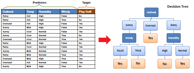
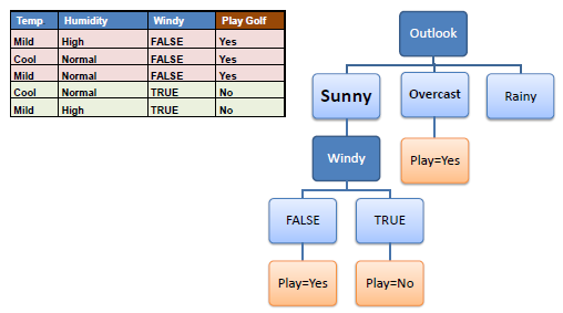
Decision tree builds classification or regression models in the form of a tree structure. It breaks down a dataset into smaller subsets with increase in depth of tree. The final result is a tree with decision nodes and leaf nodes. A decision node (e.g., Outlook) has two or more branches (e.g., Sunny, Overcast and Rainy). Leaf node (e.g., Play) represents a classification or decision. The topmost decision node in a tree which corresponds to the best predictor is called root node. Decision trees can handle both categorical and numerical data.
Types of decision trees
- Categorical Variable Decision Tree: Decision Tree which has categorical target variable then it called as categorical variable decision tree.
- Continuous Variable Decision Tree: Decision Tree which has continuous target variable then it is called as Continuous Variable Decision Tree.
Important Terminology related to Decision Trees
Let?s look at the basic terminologies used with Decision trees:
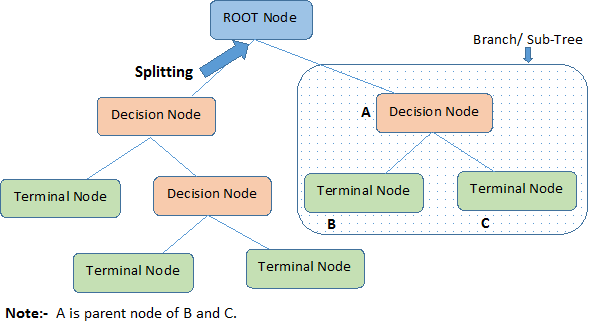
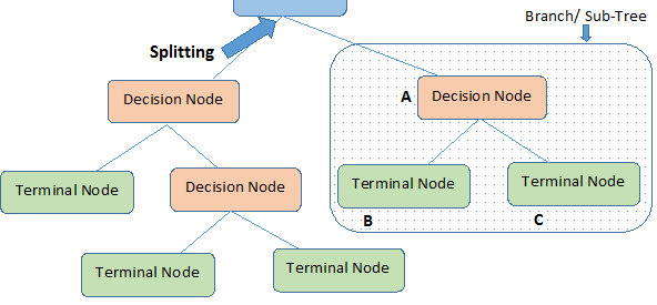
- Root Node: It represents entire population or sample and this further gets divided into two or more homogeneous sets.
- Splitting: It is a process of dividing a node into two or more sub-nodes.
- Decision Node: When a sub-node splits into further sub-nodes, then it is called decision node.
- Leaf/ Terminal Node: Nodes with no children (no further split) is called Leaf or Terminal node.
- Pruning: When we reduce the size of decision trees by removing nodes (opposite of Splitting), the process is called pruning.
- Branch / Sub-Tree: A sub section of decision tree is called branch or sub-tree.
- Parent and Child Node: A node, which is divided into sub-nodes is called parent node of sub-nodes where as sub-nodes are the child of parent node.
Algorithm used in decision trees:
- ID3
- Gini Index
- Chi-Square
- Reduction in Variance
ID3
The core algorithm for building decision trees is called ID3. Developed by J. R. Quinlan, this algorithm employs a top-down, greedy search through the space of possible branches with no backtracking. ID3 uses Entropy and Information Gain to construct a decision tree.
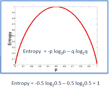
Entropy : A decision tree is built top-down from a root node and involves partitioning the data into subsets that contain instances with similar values (homogeneous). ID3 algorithm uses entropy to calculate the homogeneity of a sample. If the sample is completely homogeneous the entropy is zero and if the sample is equally divided then it has entropy of one.
To build a decision tree, we need to calculate two types of entropy using frequency tables as follows:
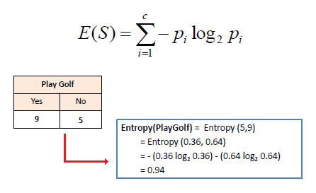
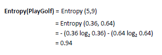
a) Entropy using the frequency table of one attribute:
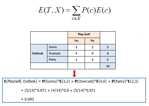
b) Entropy using the frequency table of two attributes:
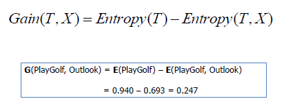
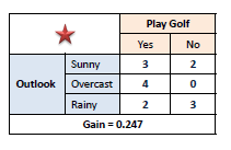
Information Gain: The information gain is based on the decrease in entropy after a data-set is split on an attribute. Constructing a decision tree is all about finding attribute that returns the highest information gain (i.e., the most homogeneous branches).
Step 1: Calculate entropy of the target.
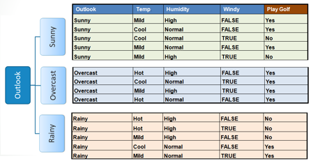
Step 2: The dataset is then split on the different attributes. The entropy for each branch is calculated. Then it is added proportionally, to get total entropy for the split. The resulting entropy is subtracted from the entropy before the split. The result is the Information Gain, or decrease in entropy.
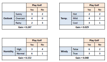
Step 3: Choose attribute with the largest information gain as the decision node, divide the dataset by its branches and repeat the same process on every branch.
Step 4a: A branch with entropy of 0 is a leaf node.
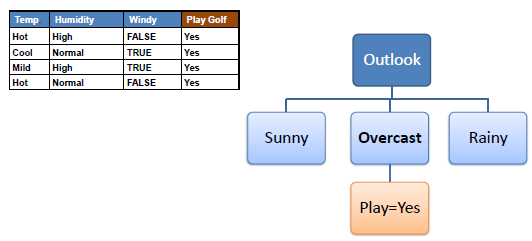
Step 4b: A branch with entropy more than 0 needs further splitting.
Step 5: The ID3 algorithm is run recursively on the non-leaf branches, until all data is classified.
Gini Index
Gini index says, if we select two items from a population at random then they must be of same class and probability for this is 1 if population is pure.
- It works with categorical target variable ?Success? or ?Failure?.
- It performs only Binary splits
- Higher the value of Gini higher the homogeneity.
- CART (Classification and Regression Tree) uses Gini method to create binary splits.
Steps to Calculate Gini for a split
- Calculate Gini for sub-nodes, using formula sum of square of probability for success and failure (p+q).
- Calculate Gini for split using weighted Gini score of each node of that split
Example: ? Referring to example where we want to segregate the students based on target variable ( playing cricket or not ). In the snapshot below, we split the population using two input variables Gender and Class. Now, I want to identify which split is producing more homogeneous sub-nodes using Gini index.
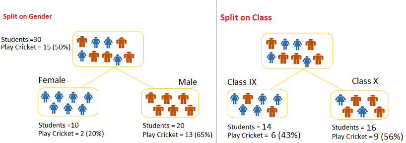
Split on Gender:
- Gini for sub-node Female = (0.2)*(0.2)+(0.8)*(0.8)=0.68
- Gini for sub-node Male = (0.65)*(0.65)+(0.35)*(0.35)=0.55
- Weighted Gini for Split Gender = (10/30)*0.68+(20/30)*0.55 = 0.59
Similar for Split on Class:
- Gini for sub-node Class IX = (0.43)*(0.43)+(0.57)*(0.57)=0.51
- Gini for sub-node Class X = (0.56)*(0.56)+(0.44)*(0.44)=0.51
- Weighted Gini for Split Class = (14/30)*0.51+(16/30)*0.51 = 0.51
Above, you can see that Gini score for Split on Gender is higher than Split on Class, hence, the node split will take place on Gender.
Chi-Square
It is an algorithm to find out the statistical significance between the differences between sub nodes and parent node. We measure it by sum of squares of standardised differences between observed and expected frequencies of target variable.
- It works with categorical target variable ?Success? or ?Failure?.
- It can perform two or more splits.
- Higher the value of Chi-Square higher the statistical significance of differences between sub-node and Parent node.
- Chi-Square of each node is calculated using formula,
- Chi-square = ((Actual ? Expected) / Expected)/2
- It generates tree called CHAID (Chi-square Automatic Interaction Detector)
Steps to Calculate Chi-square for a split:
- Calculate Chi-square for individual node by calculating the deviation for Success and Failure both
- Calculated Chi-square of Split using Sum of all Chi-square of success and Failure of each node of the split
Example: Let?s work with above example that we have used to calculate Gini.
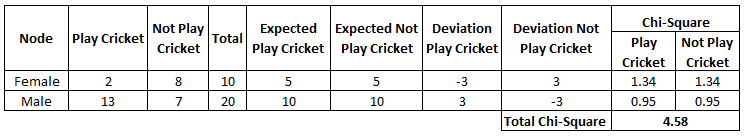
Split on Gender:
- First we are populating for node Female, Populate the actual value for ?Play Cricket? and ?Not Play Cricket?, here these are 2 and 8 respectively.
- Calculate expected value for ?Play Cricket? and ?Not Play Cricket?, here it would be 5 for both because parent node has probability of 50% and we have applied same probability on Female count(10).
- Calculate deviations by using formula, Actual ? Expected. It is for ?Play Cricket? (2?5 = -3) and for ?Not play cricket? ( 8?5 = 3).
- Calculate Chi-square of node for ?Play Cricket? and ?Not Play Cricket? using formula with formula, = ((Actual ? Expected) / Expected)/2. You can refer below table for calculation.
- Follow similar steps for calculating Chi-square value for Male node.
- Now add all Chi-square values to calculate Chi-square for split Gender.
Split on Class:
Perform similar steps of calculation for split on Class and you will come up with below table.
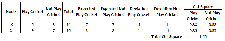
Above, you can see that Chi-square also identify the Gender split is more significant compare to Class.
Reduction in Variance
Till now, we have discussed the algorithms for categorical target variable. Reduction in variance is an algorithm used for continuous target variables (regression problems). This algorithm uses the standard formula of variance to choose the best split. The split with lower variance is selected as the criteria to split the population:
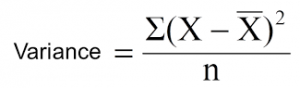
Above X-bar is mean of the values, X is actual and n is number of values.
Steps to calculate Variance:
- Calculate variance for each node.
- Calculate variance for each split as weighted average of each node variance.
Example:- Let?s assign numerical value 1 for play cricket and 0 for not playing cricket. Now follow the steps to identify the right split:
- Variance for Root node, here mean value is (15*1 + 15*0)/30 = 0.5 and we have 15 one and 15 zero. Now variance would be ((1?0.5)+(1?0.5)+?.15 times+(0?0.5)+(0?0.5)+?15 times) / 30, this can be written as (15*(1?0.5)+15*(0?0.5)) / 30 = 0.25
- Mean of Female node = (2*1+8*0)/10=0.2 and Variance = (2*(1?0.2)+8*(0?0.2)) / 10 = 0.16
- Mean of Male Node = (13*1+7*0)/20=0.65 and Variance = (13*(1?0.65)+7*(0?0.65)) / 20 = 0.23
- Variance for Split Gender = Weighted Variance of Sub-nodes = (10/30)*0.16 + (20/30) *0.23 = 0.21
- Mean of Class IX node = (6*1+8*0)/14=0.43 and Variance = (6*(1?0.43)+8*(0?0.43)) / 14= 0.24
- Mean of Class X node = (9*1+7*0)/16=0.56 and Variance = (9*(1?0.56)+7*(0?0.56)) / 16 = 0.25
- Variance for Split Gender = (14/30)*0.24 + (16/30) *0.25 = 0.25
Above, you can see that Gender split has lower variance compare to parent node, so the split would take place on Gender variable.
Until here, we learnt about the basics of decision trees and the decision making process involved to choose the best splits in building a tree model. As I said, decision tree can be applied both on regression and classification problems. Let?s understand these aspects in detail.
C4.5 algoritham
C4.5 builds decision trees from a set of training data in the same way as ID3, using the concept of information entropy.
The training data is a set of already classified samples. Each sample consists of a p-dimensional vector , where the represent attribute values or features of the sample, as well as the class in which falls.
At each node of the tree, C4.5 chooses the attribute of the data that most effectively splits its set of samples into subsets enriched in one class or the other. The splitting criterion is the normalized information gain (difference in entropy).
The attribute with the highest normalized information gain is chosen to make the decision. The C4.5 algorithm then recurs on the smaller sublists.
This algorithm has a few base cases.
All the samples in the list belong to the same class. When this happens, it simply creates a leaf node for the decision tree saying to choose that class.
None of the features provide any information gain. In this case, C4.5 creates a decision node higher up the tree using the expected value of the class.
Instance of previously-unseen class encountered. Again, C4.5 creates a decision node higher up the tree using the expected value.
C4.5 made a number of improvements to ID3. Some of these are:
Handling both continuous and discrete attributes ? In order to handle continuous attributes, C4.5 creates a threshold and then splits the list into those whose attribute value is above the threshold and those that are less than or equal to it.
Handling training data with missing attribute values ? C4.5 allows attribute values to be marked as ? for missing. Missing attribute values are simply not used in gain and entropy calculations. Handling attributes with differing costs.
Pruning trees after creation ? C4.5 goes back through the tree once it?s been created and attempts to remove branches that do not help by replacing them with leaf nodes.
Pruning:
One of the questions that arises in a decision tree algorithm is the optimal size of the final tree. A tree that is too large risks overfitting the training data and poorly generalizing to new samples. A small tree might not capture important structural information about the sample space. However,
it is hard to tell when a tree algorithm should stop because it is impossible to tell if the addition of a single extra node will dramatically decrease error. This problem is known as the horizon effect.
A common strategy is to grow the tree until each node contains a small number of instances then use pruning to remove nodes that do not provide additional information.
Pruning should reduce the size of a learning tree without reducing predictive accuracy as measured by a cross-validation set. There are many techniques for tree pruning that differ in the measurement that is used to optimize performance.
Reduced error pruning
One of the simplest forms of pruning is reduced error pruning. Starting at the leaves, each node is replaced with its most popular class. If the prediction accuracy is not affected then the change is kept. While somewhat naive, reduced error pruning has the advantage of simplicity and speed.
Cost complexity pruning
Cost complexity pruning generates a series of trees T0 . . . Tm where T0 is the initial tree and Tm is the root alone. At step i the tree is created by removing a subtree from tree i-1and replacing it with a leaf node with value chosen as in the tree building algorithm. The subtree that is removed is chosen as follows. Define the error rate of tree T over data set S as err(T,S). The subtree that minimizes is chosen for removal. The function prune(T,t) defines the tree gotten by pruning the subtrees t from the tree T. Once the series of trees has been created, the best tree is chosen by generalized accuracy as measured by a training set or cross-validation.
Advantages:
Decision trees assist managers in evaluating upcoming choices. The tree creates a visual representation of all possible outcomes, rewards and follow-up decisions in one document. Each subsequent decision resulting from the original choice is also depicted on the tree, so you can see the overall effect of any one decision. As you go through the tree and make choices, you will see a specific path from one node to another and the impact a decision made now could have down the road.
- Brainstorming Outcomes : Decision trees help you think of all possible outcomes for an upcoming choice. The consequences of each outcome must be fully explored, so no details are missed. Taking the time to brainstorm prevents overreactions to any one variable. The graphical depiction of various alternatives makes them easier to compare with each other. The decision tree also adds transparency to the process. An independent party can see exactly how a particular decision was made.
- Decision Tree Versatility : Decision trees can be customized for a variety for situations. The logical form is good for programmers and engineers. Technicians can also use decision trees to diagnose mechanical failures in equipment or troubleshoot auto repairs. Decision trees are also helpful for evaluating business or investment alternatives. Managers can recreate the math used in a particular decision tree to analyzing the company?s decision-making process.
- Less data cleaning required: It requires less data cleaning compared to some other modeling techniques. It is not influenced by outliers and missing values to a fair degree.
- Data type is not a constraint: It can handle both numerical and categorical variables.
- Non Parametric Method: Decision tree is considered to be a non-parametric method. This means that decision trees have no assumptions about the space distribution and the classifier structure.
