 A bug in the code is worth two in the documentation.
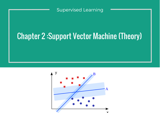
Welcome to the second stepping stone of Supervised Machine Learning. Again, this chapter is divided into two parts. Part 1 (this one) discusses about theory, working and tuning parameters. Part 2 (here) we take on small coding exercise challenge.
If you haven?t read the Naive Bayes, I would suggest you to read it thorough here.
0. Introduction
A Support Vector Machine (SVM) is a discriminative classifier formally defined by a separating hyperplane. In other words, given labeled training data (supervised learning), the algorithm outputs an optimal hyperplane which categorizes new examples. In two dimentional space this hyperplane is a line dividing a plane in two parts where in each class lay in either side.
Confusing? Don?t worry, we shall learn in laymen terms.
Suppose you are given plot of two label classes on graph as shown in image (A). Can you decide a separating line for the classes?
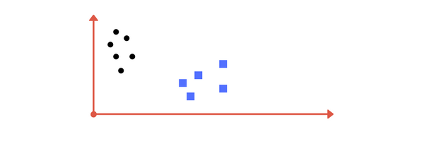 Image A: Draw a line that separates black circles and blue squares.
You might have come up with something similar to following image (image B). It fairly separates the two classes. Any point that is left of line falls into black circle class and on right falls into blue square class. Separation of classes. That?s what SVM does. It finds out a line/ hyper-plane (in multidimensional space that separate outs classes). Shortly, we shall discuss why I wrote multidimensional space.
 s Image B: Sample cut to divide into two classes.
1. Making it a Bit complex?
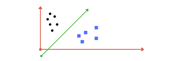
So far so good. Now consider what if we had data as shown in image below? Clearly, there is no line that can separate the two classes in this x-y plane. So what do we do? We apply transformation and add one more dimension as we call it z-axis. Lets assume value of points on z plane, w = x + y. In this case we can manipulate it as distance of point from z-origin. Now if we plot in z-axis, a clear separation is visible and a line can be drawn .
 Can you draw a separating line in this plane?
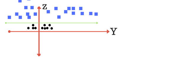 plot of zy axis. A separation can be made here.
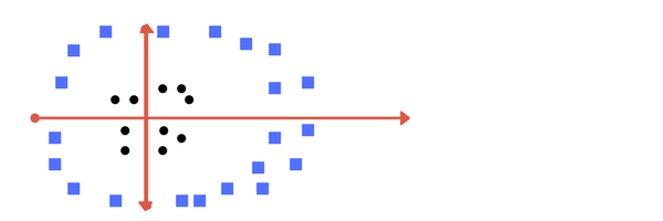
When we transform back this line to original plane, it maps to circular boundary as shown in image E. These transformations are called kernels.
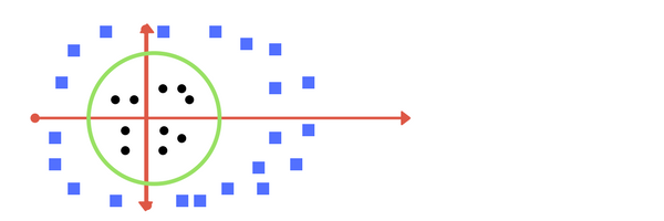 Transforming back to x-y plane, a line transforms to circle.
Thankfully, you don?t have to guess/ derive the transformation every time for your data set. The sklearn library’s SVM implementation provides it inbuilt.
2. Making it a little more complex?
What if data plot overlaps? Or, what in case some of the black points are inside the blue ones? Which line among 1 or 2?should we draw?
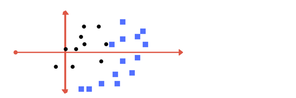 What in this case?
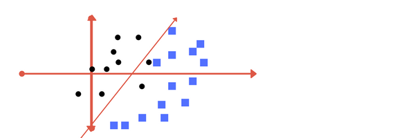 Image 1
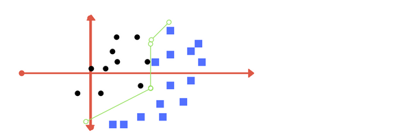 Image 2
Which one do you think? Well, both the answers are correct. The first one tolerates some outlier points. The second one is trying to achieve 0 tolerance with perfect partition.
But, there is trade off. In real world application, finding perfect class for millions of training data set takes lot of time. As you will see in coding. This is called regularization parameter. In next section, we define two terms regularization parameter and gamma. These are tuning parameters in SVM classifier. Varying those we can achive considerable non linear classification line with more accuracy in reasonable amount of time. In coding exercise (part 2 of this chapter) we shall see how we can increase the accuracy of SVM by tuning these parameters.
One more parameter is kernel. It defines whether we want a linear of linear separation. This is also discussed in next section.
 When somebody asks me for advice.
3. Tuning parameters: Kernel, Regularization, Gamma and Margin.
Kernel
The learning of the hyperplane in linear SVM is done by transforming the problem using some linear algebra. This is where the kernel plays role.
For linear kernel the equation for prediction for a new input using the dot product between the input (x) and each support vector (xi) is calculated as follows:
f(x) = B(0) + sum(ai * (x,xi))
This is an equation that involves calculating the inner products of a new input vector (x) with all support vectors in training data. The coefficients B0 and ai (for each input) must be estimated from the training data by the learning algorithm.
The polynomial kernel can be written as K(x,xi) = 1 + sum(x * xi)^d and exponential as K(x,xi) = exp(-gamma * sum((x ? xi)). [Source for this excerpt : http://machinelearningmastery.com/].
Polynomial and exponential kernels calculates separation line in higher dimension. This is called kernel trick
Regularization
The Regularization parameter (often termed as C parameter in python?s sklearn library) tells the SVM optimization how much you want to avoid misclassifying each training example.
For large values of C, the optimization will choose a smaller-margin hyperplane if that hyperplane does a better job of getting all the training points classified correctly. Conversely, a very small value of C will cause the optimizer to look for a larger-margin separating hyperplane, even if that hyperplane misclassifies more points.
The images below (same as image 1 and image 2 in section 2) are example of two different regularization parameter. Left one has some misclassification due to lower regularization value. Higher value leads to results like right one.
Left: low regularization value, right: high regularization value
Gamma
The gamma parameter defines how far the influence of a single training example reaches, with low values meaning ?far? and high values meaning ?close?. In other words, with low gamma, points far away from plausible seperation line are considered in calculation for the seperation line. Where as high gamma means the points close to plausible line are considered in calculation.
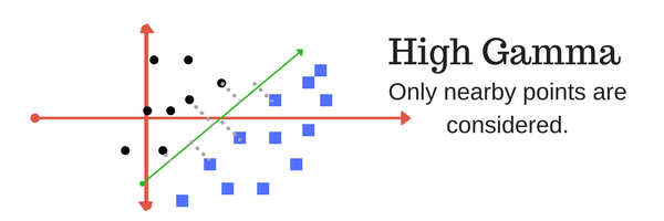 High Gamma
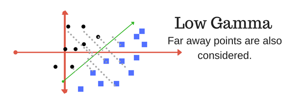 Low Gamma
Margin
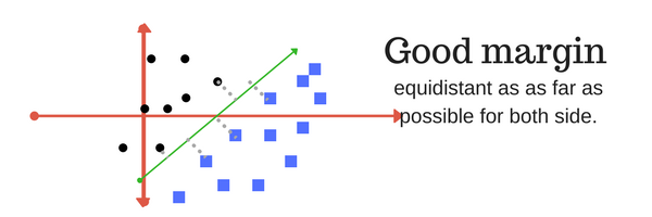
And finally last but very importrant characteristic of SVM classifier. SVM to core tries to achieve a good margin.
A margin is a separation of line to the closest class points.
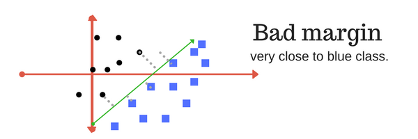
A good margin is one where this separation is larger for both the classes. Images below gives to visual example of good and bad margin. A good margin allows the points to be in their respective classes without crossing to other class.
4. In next part of this chapter,
In next part (here) we shall tweak and play tuning parameters and implement a mini project for SVM classifier (also known as SVC) using python?s sklearn library. We shall compare the results with the Naive Bayes Classfier. Check out coding part here : https://medium.com/machine-learning-101/chapter-2-svm-support-vector-machine-coding-edd8f1cf8f2d.
5. Conclusion
I hope that this section was helpful in understanding the working behind SVM classifier. Comment down your thoughts, feedback or suggestions if any below. If you liked this post, share it with your friends, subscribe to Machine Learning 101 click the heart(?) icon. Peace!
 Coding is but art of thinking than typing.

 — Theory)
 — Theory)