In this tutorial we are going to explain, one of the emerging and prominent word embedding technique called Word2Vec proposed by Mikolov et al. in 2013. We have collected these content from different tutorials and sources to facilitate readers in a single place. I hope it helps.
1. Overview of Word2Vec
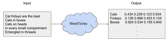
Word2vec is a combination of models used to represent distributed representations of words in a corpus C. Word2Vec (W2V) is an algorithm that accepts text corpus as an input and outputs a vector representation for each word, as shown in the diagram below:
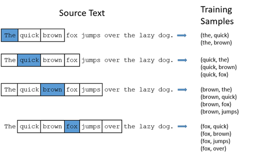
There are two flavors of this algorithm namely: CBOW and Skip-Gram. Given a set of sentences (also called corpus) the model loops on the words of each sentence and either tries to use the current word w in order to predict its neighbors (i.e., its context), this approach is called ?Skip-Gram?, or it uses each of these contexts to predict the current word w, in that case the method is called ?Continuous Bag Of Words? (CBOW). To limit the number of words in each context, a parameter called ?window size? is used.
The vectors we use to represent words are called neural word embeddings, and representations are strange. One thing describes another, even though those two things are radically different. As Elvis Costello said: ?Writing about music is like dancing about architecture.? Word2vec ?vectorizes? about words, and by doing so it makes natural language computer-readable ? we can start to perform powerful mathematical operations on words to detect their similarities.
So, a neural word embedding represents a word with numbers. It?s a simple, yet unlikely, translation. Word2vec is similar to an autoencoder, encoding each word in a vector, but rather than training against the input words through reconstruction, as a restricted Boltzmann machine does, word2vec trains words against other words that neighbor them in the input corpus.
It does so in one of two ways, either using context to predict a target word (a method known as continuous bag of words, or CBOW), or using a word to predict a target context, which is called skip-gram. We use the latter method because it produces more accurate results on large datasets.
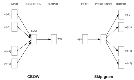
When the feature vector assigned to a word cannot be used to accurately predict that word?s context, the components of the vector are adjusted. Each word?s context in the corpus is the teacher sending error signals back to adjust the feature vector. The vectors of words judged similar by their context are nudged closer together by adjusting the numbers in the vector. In this tutorial, we are going to focus on Skip-Gram model which in contrast to CBOW consider center word as input as depicted in figure above and predict context words.
2. Model overview
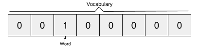
We understood that we have to feed some strange neural network with some pairs of words but we can?t just do that using as inputs the actual characters, we have to find some way to represent these words mathematically so that the network can process them. One way to do this is to create a vocabulary of all the words in our text and then to encode our word as a vector of the same dimensions of our vocabulary. Each dimension can be thought as a word in our vocabulary. So we will have a vector with all zeros and a 1 which represents the corresponding word in the vocabulary. This encoding technique is called one-hot encoding. Considering our example, if we have a vocabulary made out of the words ?the?, ?quick?, ?brown?, ?fox?, ?jumps?, ?over?, ?the? ?lazy?, ?dog?, the word ?brown? is represented by this vector: [ 0, 0, 1, 0, 0, 0 ,0 ,0 ,0 ].
The Skip-gram model takes in a corpus of text and creates a hot-vector for each word. A hot vector is a vector representation of a word where the vector is the size of the vocabulary (total unique words). All dimensions are set to 0 except the dimension representing the word that is used as an input at that point in time. Here is an example of a hot vector:
The above input is given to a neural network with a single hidden layer.
We?re going to represent an input word like ?ants? as a one-hot vector. This vector will have 10,000 components (one for every word in our vocabulary) and we?ll place a ?1? in the position corresponding to the word ?ants?, and 0s in all of the other positions. The output of the network is a single vector (also with 10,000 components) containing, for every word in our vocabulary, the probability that a randomly selected nearby word is that vocabulary word.
In word2vec, a distributed representation of a word is used. Take a vector with several hundred dimensions (say 1000). Each word is represented by a distribution of weights across those elements. So instead of a one-to-one mapping between an element in the vector and a word, the representation of a word is spread across all the elements in the vector, and each element in the vector contributes to the definition of many words.
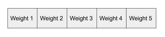
If I label the dimensions in a hypothetical word vector (there are no such pre-assigned labels in the algorithm of course), it might look a bit like this:
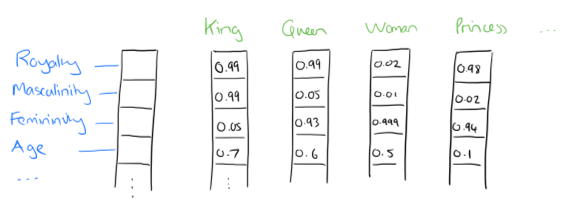
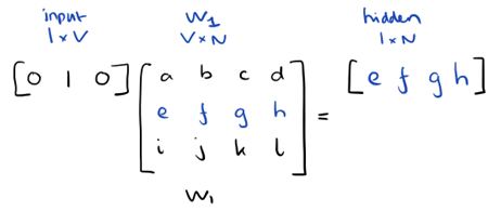
Such a vector comes to represent in some abstract way the ?meaning? of a word. And as we?ll see next, simply by examining a large corpus it?s possible to learn word vectors that are able to capture the relationships between words in a surprisingly expressive way. We can also use the vectors as inputs to a neural network. Since our input vectors are one-hot, multiplying an input vector by the weight matrix W1 amounts to simply selecting a row from W1.
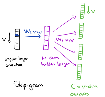
From the hidden layer to the output layer, the second weight matrix W2 can be used to compute a score for each word in the vocabulary, and softmax can be used to obtain the posterior distribution of words. The skip-gram model is the opposite of the CBOW model. It is constructed with the focus word as the single input vector, and the target context words are now at the output layer. The activation function for the hidden layer simply amounts to copying the corresponding row from the weights matrix W1 (linear) as we saw before. At the output layer, we now output C multinomial distributions instead of just one. The training objective is to mimimize the summed prediction error across all context words in the output layer. In our example, the input would be ?learning?, and we hope to see (?an?, ?efficient?, ?method?, ?for?, ?high?, ?quality?, ?distributed?, ?vector?) at the output layer.
Here?s the architecture of our neural network.
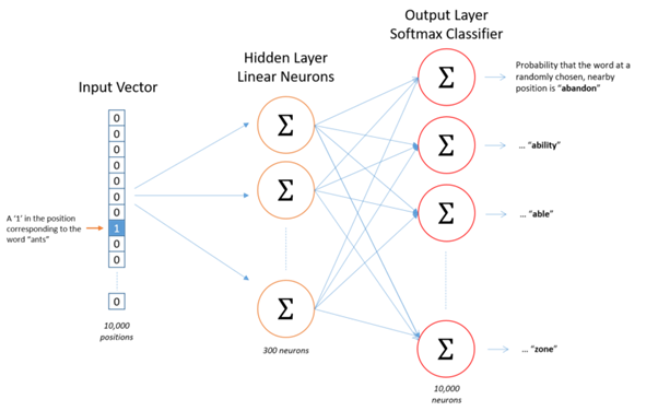
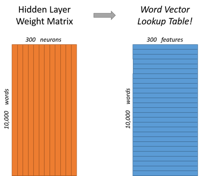
For our example, we?re going to say that we?re learning word vectors with 300 features. So the hidden layer is going to be represented by a weight matrix with 10,000 rows (one for every word in our vocabulary) and 300 columns (one for every hidden neuron). 300 features is what Google used in their published model trained on the Google news dataset (you can download it from here). The number of features is a ?hyper parameter? that you would just have to tune to your application (that is, try different values and see what yields the best results).
If you look at the rows of this weight matrix, these are what will be our word vectors!
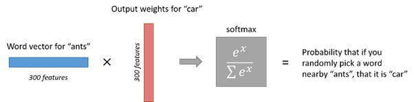
So the end goal of all of this is really just to learn this hidden layer weight matrix ? the output layer we?ll just toss when we?re done! The 1 x 300 word vector for ?ants? then gets fed to the output layer. The output layer is a softmax regression classifier. Specifically, each output neuron has a weight vector which it multiplies against the word vector from the hidden layer, then it applies the function exp(x) to the result. Finally, in order to get the outputs to sum up to 1, we divide this result by the sum of the results from all 10,000 output nodes. Here?s an illustration of calculating the output of the output neuron for the word ?car?.
If two different words have very similar ?contexts? (that is, what words are likely to appear around them), then our model needs to output very similar results for these two words. And one way for the network to output similar context predictions for these two words is if the word vectors are similar. So, if two words have similar contexts, then our network is motivated to learn similar word vectors for these two words! Ta da!
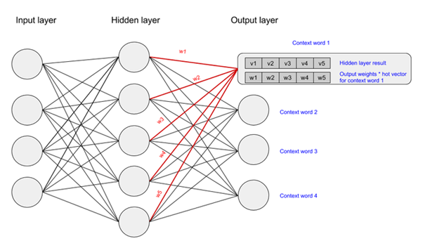
Each dimension of the input passes through each node of the hidden layer. The dimension is multiplied by the weight leading it to the hidden layer. Because the input is a hot vector, only one of the input nodes will have a non-zero value (namely the value of 1). This means that for a word only the weights associated with the input node with value 1 will be activated, as shown in the image above.
As the input in this case is a hot vector, only one of the input nodes will have a non-zero value. This means that only the weights connected to that input node will be activated in the hidden nodes. An example of the weights that will be considered is depicted below for the second word in the vocabulary:
The vector representation of the second word in the vocabulary (shown in the neural network above) will look as follows, once activated in the hidden layer:
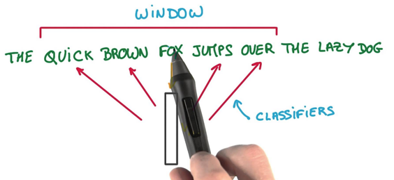
Those weights start off as random values. The network is then trained in order to adjust the weights to represent the input words. This is where the output layer becomes important. Now that we are in the hidden layer with a vector representation of the word we need a way to determine how well we have predicted that a word will fit in a particular context. The context of the word is a set of words within a window around it, as shown below:
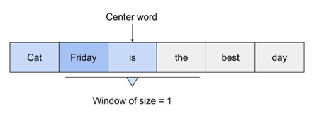
The above image shows that the context for Friday includes words like ?cat? and ?is?. The aim of the neural network is to predict that ?Friday? falls within this context.
We activate the output layer by multiplying the vector that we passed through the hidden layer (which was the input hot vector * weights entering hidden node) with a vector representation of the context word (which is the hot vector for the context word * weights entering the output node). The state of the output layer for the first context word can be visualised below:
The above multiplication is done for each word to context word pair. We then calculate the probability that a word belongs with a set of context words using the values resulting from the hidden and output layers. Lastly, we apply stochastic gradient descent to change the values of the weights in order to get a more desirable value for the probability calculated.
In gradient descent we need to calculate the gradient of the function being optimised at the point representing the weight that we are changing. The gradient is then used to choose the direction in which to make a step to move towards the local optimum, as shown in the minimisation example below.
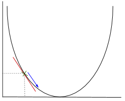
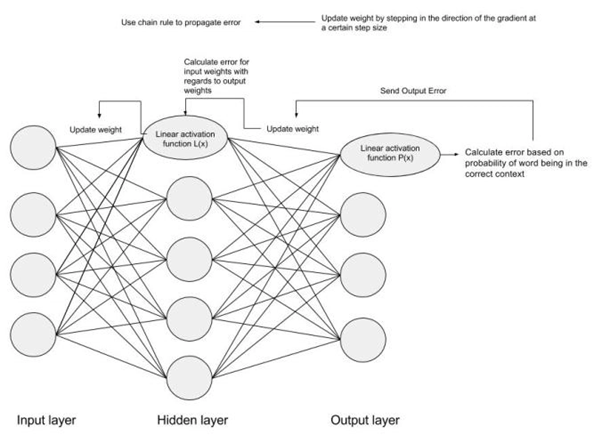
The weight will be changed by making a step in the direction of the optimal point (in the above example, the lowest point in the graph). The new value is calculated by subtracting from the current weight value the derived function at the point of the weight scaled by the learning rate. The next step is using Backpropagation, to adjust the weights between multiple layers. The error that is computed at the end of the output layer is passed back from the output layer to the hidden layer by applying the Chain Rule. Gradient descent is used to update the weights between these two layers. The error is then adjusted at each layer and sent back further. Here is a diagram to represent backpropagation:
3. Understanding using Example
Word2vec uses a single hidden layer, fully connected neural network as shown below. The neurons in the hidden layer are all linear neurons. The input layer is set to have as many neurons as there are words in the vocabulary for training. The hidden layer size is set to the dimensionality of the resulting word vectors. The size of the output layer is same as the input layer. Thus, if the vocabulary for learning word vectors consists of V words and N to be the dimension of word vectors, the input to hidden layer connections can be represented by matrix WI of size VxN with each row representing a vocabulary word. In same way, the connections from hidden layer to output layer can be described by matrix WO of size NxV. In this case, each column of WO matrix represents a word from the given vocabulary.
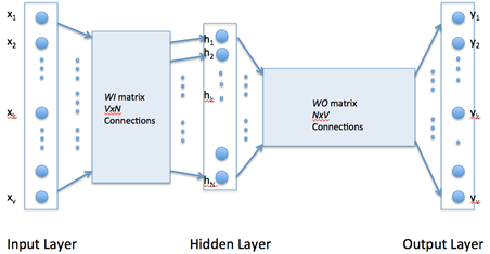
The input to the network is encoded using ?1-out of -V? representation meaning that only one input line is set to one and rest of the input lines are set to zero.
Let suppose we have a training corpus having the following sentences:
?the dog saw a cat?, ?the dog chased the cat?, ?the cat climbed a tree?
The corpus vocabulary has eight words. Once ordered alphabetically, each word can be referenced by its index. For this example, our neural network will have eight input neurons and eight output neurons. Let us assume that we decide to use three neurons in the hidden layer. This means that WI and WO will be 83 and 38 matrices, respectively. Before training begins, these matrices are initialized to small random values as is usual in neural network training. Just for the illustration sake, let us assume WI and WO to be initialized to the following values:
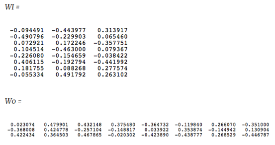
Suppose we want the network to learn relationship between the words ?cat? and ?climbed?. That is, the network should show a high probability for ?climbed? when ?cat? is inputted to the network. In word embedding terminology, the word ?cat? is referred as the context word and the word ?climbed? is referred as the target word. In this case, the input vector X will be [0 1 0 0 0 0 0 0]t. Notice that only the second component of the vector is 1. This is because the input word is ?cat? which is holding number two position in sorted list of corpus words. Given that the target word is ?climbed?, the target vector will look like [0 0 0 1 0 0 0 0 ]t. With the input vector representing ?cat?, the output at the hidden layer neurons can be computed as:
Ht = XtWI = [-0.490796 -0.229903 0.065460]
It should not surprise us that the vector H of hidden neuron outputs mimics the weights of the second row of WI matrix because of 1-out-of-Vrepresentation. So the function of the input to hidden layer connections is basically to copy the input word vector to hidden layer. Carrying out similar manipulations for hidden to output layer, the activation vector for output layer neurons can be written as
HtWO = [0.100934 -0.309331 -0.122361 -0.151399 0.143463 -0.051262 -0.079686 0.112928]
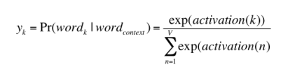
Since, the goal is produce probabilities for words in the output layer, Pr(wordk|wordcontext) for k = 1, V, to reflect their next word relationship with the context word at input, we need the sum of neuron outputs in the output layer to add to one. Word2vec achieves this by converting activation values of output layer neurons to probabilities using the softmax function. Thus, the output of the k-th neuron is computed by the following expression where activation(n) represents the activation value of the n-th output layer neuron:
Thus, the probabilities for eight words in the corpus are:
0.143073 0.094925 0.114441 0.111166 0.149289 0.122874 0.119431 0.144800
The probability in bold is for the chosen target word ?climbed?. Given the target vector [0 0 0 1 0 0 0 0 ]t, the error vector for the output layer is easily computed by subtracting the probability vector from the target vector. Once the error is known, the weights in the matrices WO and WI can be updated using backpropagation. Thus, the training can proceed by presenting different context-target words pair from the corpus. This is how Word2vec learns relationships between words and in the process develops vector representations for words in the corpus.
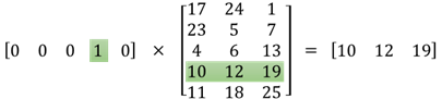
The idea behind word2vec is to represent words by a vector of real numbers of dimension d. Therefore the second matrix is the representation of those words. The i-th line of this matrix is the vector representation of the i-th word. Let?s say that in your example you have 5 words : [?Lion?, ?Cat?, ?Dog?, ?Horse?, ?Mouse?], then the first vector [0,0,0,1,0] means you?re considering the word ?Horse? and so the representation of ?Horse? is [10, 12, 19]. Similarly, [17, 24, 1] is the representation of the word ?Lion?.
To my knowledge, there are no ?human meaning? specifically to each of the numbers in these representations. One number is not representing if the word is a verb or not, an adjective or not? It?s just the weights that you change to solve your optimization problem to learn the representation of your words.
A visual diagram best elaborating word2vec matrix multiplication process is depicted in following figure:
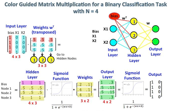
The first matrix represents the input vector in one hot format. The second matrix represents the synaptic weights from the input layer neurons to the hidden layer neurons. Especially notice the left top corner where the Input Layer matrix is multiplied with the Weight matrix. Now look at the top right. This matrix multiplication InputLayer dot-producted with Weights Transpose is just a handy way to represent the neural network at the top right.
The first part, [0 0 0 1 0 ? 0] represents the input word as a one hot vector and the other matrix represents the weight for the connection of each of the input layer neurons to the hidden layer neurons. As Word2Vec trains, it backpropagates (using gradient descent) into these weights and changes them to give better representations of words as vectors. Once training is accomplished, you use only this weight matrix, take [0 0 1 0 0 ? 0] for say ?dog? and multiply it with the improved weight matrix to get the vector representation of ?dog? in a dimension = no of hidden layer neurons. In the diagram, the number of hidden layer neurons is 3.
In a nutshell, Skip-gram model reverses the use of target and context words. In this case, the target word is fed at the input, the hidden layer remains the same, and the output layer of the neural network is replicated multiple times to accommodate the chosen number of context words. Taking the example of ?cat? and ?tree? as context words and ?climbed? as the target word, the input vector in the skim-gram model would be [0 0 0 1 0 0 0 0 ]t, while the two output layers would have [0 1 0 0 0 0 0 0] t and [0 0 0 0 0 0 0 1 ]t as target vectors respectively. In place of producing one vector of probabilities, two such vectors would be produced for the current example. The error vector for each output layer is produced in the manner as discussed above. However, the error vectors from all output layers are summed up to adjust the weights via backpropagation. This ensures that weight matrix WO for each output layer remains identical all through training.
We need few additional modifications to the basic skip-gram model which are important for making it feasible to train. Running gradient descent on a neural network that large is going to be slow. And to make matters worse, you need a huge amount of training data to tune that many weights and avoid over-fitting. millions of weights times billions of training samples means that training this model is going to be a beast. For that, authors have proposed two techniques called subsampling and negative sampling in which insignificant words are removed and only a specific sample of weights are updated.
Mikolov et al. also use a simple subsampling approach to counter the imbalance between rare and frequent words in the training set (for example, ?in?, ?the?, and ?a? provide less information value than rare words). Each word in the training set is discarded with probability P(wi) where
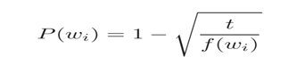
f(wi) is the frequency of word wi and t is a chosen threshold, typically around 10?5.
4. Implementation details
Word2vec has been implemented in various languages but here we will focus especially on Java i.e., DeepLearning4j [6], darks-learning [10] and python [7][8][9]. Various neural net algorithms have been implemented in DL4j, code is available on GitHub.
To implement it in DL4j, we will go through few steps given as following:
a) Word2Vec Setup
Create a new project in IntelliJ using Maven. Then specify properties and dependencies in the POM.xml file in your project?s root directory.
b) Load data
Now create and name a new class in Java. After that, you?ll take the raw sentences in your .txt file, traverse them with your iterator, and subject them to some sort of pre-processing, such as converting all words to lowercase.
String filePath = new ClassPathResource(?raw_sentences.txt?).getFile().getAbsolutePath();
log.info(?Load & Vectorize Sentences?.?);
// Strip white space before and after for each line
SentenceIterator iter = new BasicLineIterator(filePath);
If you want to load a text file besides the sentences provided in our example, you?d do this:
log.info(“Load data….”);SentenceIterator iter = new LineSentenceIterator(new File(“/Users/cvn/Desktop/file.txt”));iter.setPreProcessor(new SentencePreProcessor() {@Overridepublic String preProcess(String sentence) {return sentence.toLowerCase();}});
c) Tokenizing the Data
Word2vec needs to be fed words rather than whole sentences, so the next step is to tokenize the data. To tokenize a text is to break it up into its atomic units, creating a new token each time you hit a white space, for example.
// Split on white spaces in the line to get wordsTokenizerFactory t = new DefaultTokenizerFactory();t.setTokenPreProcessor(new CommonPreprocessor());
d) Training the Model
Now that the data is ready, you can configure the Word2vec neural net and feed in the tokens.
log.info(“Building model….”);Word2Vec vec = new Word2Vec.Builder().minWordFrequency(5).layerSize(100).seed(42).windowSize(5).iterate(iter).tokenizerFactory(t).build();log.info(“Fitting Word2Vec model….”);vec.fit();
This configuration accepts several hyperparameters. A few require some explanation:
- batchSize is the amount of words you process at a time.
- minWordFrequency is the minimum number of times a word must appear in the corpus. Here, if it appears less than 5 times, it is not learned. Words must appear in multiple contexts to learn useful features about them. In very large corpora, it?s reasonable to raise the minimum.
- useAdaGrad ? Adagrad creates a different gradient for each feature. Here we are not concerned with that.
- layerSize specifies the number of features in the word vector. This is equal to the number of dimensions in the featurespace. Words represented by 500 features become points in a 500-dimensional space.
- learningRate is the step size for each update of the coefficients, as words are repositioned in the feature space.
- minLearningRate is the floor on the learning rate. Learning rate decays as the number of words you train on decreases. If learning rate shrinks too much, the net?s learning is no longer efficient. This keeps the coefficients moving.
- iterate tells the net what batch of the dataset it?s training on.
- tokenizer feeds it the words from the current batch.
- vec.fit() tells the configured net to begin training.
e) Evaluating the Model, Using Word2vec
The next step is to evaluate the quality of your feature vectors.
// Write word vectorsWordVectorSerializer.writeWordVectors(vec, “pathToWriteto.txt”);log.info(“Closest Words:”);Collection<String> lst = vec.wordsNearest(“day”, 10);System.out.println(lst);UiServer server = UiServer.getInstance();System.out.println(“Started on port ” + server.getPort());//output: [night, week, year, game, season, during, office, until, -]
The line vec.similarity(“word1″,”word2”) will return the cosine similarity of the two words you enter. The closer it is to 1, the more similar the net perceives those words to be (see the Sweden-Norway example above). For example:
double cosSim = vec.similarity(“day”, “night”);System.out.println(cosSim);//output: 0.7704452276229858
With vec.wordsNearest(“word1”, numWordsNearest), the words printed to the screen allow you to eyeball whether the net has clustered semantically similar words. You can set the number of nearest words you want with the second parameter of wordsNearest. For example:
Collection<String> lst3 = vec.wordsNearest(“man”, 10);System.out.println(lst3);//output: [director, company, program, former, university, family, group, such, general]
5. References
1) http://mccormickml.com/2016/04/27/word2vec-resources/
2) https://towardsdatascience.com/word2vec-skip-gram-model-part-1-intuition-78614e4d6e0b
3) https://deeplearning4j.org/docs/latest/deeplearning4j-nlp-word2vec
4) https://intothedepthsofdataengineering.wordpress.com/2017/06/26/an-overview-of-word2vec/
5) https://blog.acolyer.org/2016/04/21/the-amazing-power-of-word-vectors/
6) Word2vec in Java in http://deeplearning4j.org/word2vec.html
7) Word2Vec and Doc2Vec in Python in genism http://radimrehurek.com/2013/09/deep-learning-with-word2vec-and-gensim/
8) http://rare-technologies.com/word2vec-tutorial/
9) https://www.tensorflow.org/versions/r0.8/tutorials/word2vec/index.html
10) https://www.programcreek.com/java-api-examples/index.php?source_dir=darks-learning-master/src/main/java/darks/learning/word2vec/Word2Vec.java