As an information designer, I?m charged with summarizing data. But even the simplest of questions, like ?How big is a typical case?? presents choices about what to do; about what kind of summary to use. An ?average? is supposed to describe something like a typical case, or the ?central tendency? of the data. But there are many kinds of averages, as you might know. Here I?ll give a quick overview of two familiar averages, median and arithmetic mean, and compare them to a third, the geometric mean ? which I think should get a lot more use than it does.
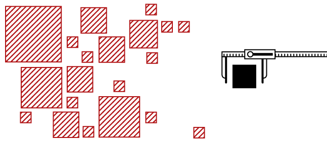
To help illustrate each of the statistics, I?ll use a small example dataset throughout the article:

The Median
This is when you select the middle element of your data, after ordering them from small to large (and if there?s an even number, take the arithmetic mean of the two closest to the middle). In our example this is 2:

Medians are useful for dividing the data into two halves, each with the same number of elements ? e.g. ?big? and ?small? bins. The median is really a special case of a quantile: it?s the 50th percentile (50/100), or second quartile (2/4), which means it can easily be paired with other quantiles, like it with box-and-whisker plots.
Extreme Values
An advantage of medians is that they ignore extreme values. This can be helpful, but in my experience, people want to ignore extremes far too readily: they categorize anything inconvenient to their pet theory as an ?outlier? and delete it. But extremes help to tell you what?s possible, and could suggest a very different distribution in your data from what you expect. Be cautious about fooling yourself.
In fact, medians don?t just ignore outliers? values: they ignore the values of everything, except from the middle element. Otherwise, only rank order matters. The perils of this can be seen in the example: 44% of the elements are 9s, but that value does not affect the median: the 9s could be anything, even 1 million each, and the median would remain 2.
It?s hard to go truly wrong by using medians as your summary statistic: they work on many kinds of data, and are robust with respect to outliers. But because they ignore so much of the data, they don?t work well with small sets of data. And they can?t be used well as part of ratios or many other other manipulations ? as we?ll see shortly.
The Arithmetic Mean
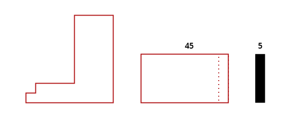
You would usually just call this the ?mean? or, if you?re sloppy with words, the ?average? (like Microsoft Excel does): add everything up and divide by the number of elements. These steps effectively spread the total value you have across all the cases you have, which makes all cases the same. Basically, you are answering the question ?What would each case have to be, if all cases were identical??
You can also look at the mean calculation geometrically: the mean effectively reconfigures separate areas into one big area, and then cuts it into equal parts:
Compared to the median, the mean has a real advantage: it takes account of all values, and is much less likely to jump around if you add in a data point or two (unless they?re extreme).
Make Sure it Makes Sense
An important proviso is that the quantities you?re averaging have to be ?addable? in some sensical way, given the real-world meaning of your data. Usually, this is no big deal: you can almost always find some valid interpretation of the arithmetic mean. The question is whether it?s the interpretation you want ? because alternative statistics can produce other reasonable results at the same time, and you have to decide.
The ?Trick? Grandma Problem
A common sort of math problem tries to lull students into taking an arithmetic mean when they shouldn?t: ?You drive at 40 mph to Grandma?s house, and then 60 mph back; what was your average speed?? The naive student writes 50, ignoring the ?mph? as much as possible, and treating the values as distances. The trick is that time is hidden in the units, but actually changes between the two legs of the journey. To get at the desired answer, the legs must be weighted differently, either with a weighted mean (some values are effectively duplicated to count for more), or a harmonic mean (which I won?t discuss in this article). Because we?re really dealing with rates, with a ?per hour? in there, additive combination no longer makes sense. Another moral is to pay attention to units.
(Some people, in explaining the problem above, will proclaim that harmonic means should always be used for averaging rates. But nothing of the sort is true: it depends on whether time or distance vary, and on what you?re interested in. Beware blanket rules, especially from the internet, except for this one!)
The Geometric Mean
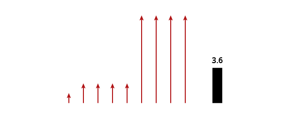
The operation here parallels that for the arithmetic mean, but we combine our values with a product instead of a sum, and then split them up again with a root. The conceptual difference is seeing each data point as a scaling factor, which combine by increasing each other multiplicatively. In our example data, we have: 1 x 2 x 2 x 2 x 2 x 9 x 9 x 9 x 9 = 104,976; and the 9th root of that yields about 3.6.
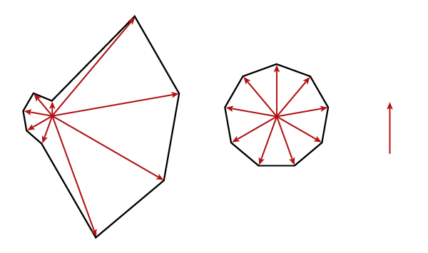
There is also a spatial interpretation of this, it?s a little but harder: each item extends a volume into another dimension, for 9 dimensions total. We then squish this hyper-volume into into a squarish shape so that every edge is the same, and measure an edge. That is, the average is what any scaling factor would be, if they were all the same.
If that seems too abstract, try to imagine what happens with just three data points, which is analogous: we?d measure the length, height, and width of a rectangular object, squish it into a cube, and measure one side of it. We can?t illustrate this well on paper, or pixels, but here is a crude illustration:
The big assumption of the geometric mean is that the data can really be interpreted as scaling factors: there can?t be zeros or negative numbers, which don?y really apply. (You can, technically, calculate it with zeros, but then the result will also be 0; not very informative.) Some computer applications may also break when you take the product of a large dataset, from lack of memory. But fear not, you can do the algorithm in reverse order, with roots first and product second.
I?m a fan of the geometric mean, and it has many advantages and good uses. I?ll discuss a handful below ? many are really saying similar things, but in different contexts, for different goals.
Skewed Data
In the real world, data are often skewed downward, with a lot of small values, and a few large ones. (For instance: the commonness of species in a forest, salaries in a corporation, distance of trips taken in your car.) If this is what you have, the arithmetic mean will fail, and fail spectacularly, to describe the ?central tendency? ? you need the geometric mean instead.
Consider what happens if we modify our example dataset to make the final value an extreme outlier of 90 instead of 9, thus making most of our values comparatively very small:
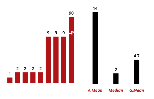
We can see how the arithmetic mean is highly sensitive to this one outlier: it now suggests that a ?typical? value is 14, even when just one item reaches that level. Extreme insensitivity to the outlier is seen in the median: it still computes to 2, despite this big change. The geometric mean offers a compromise: it shifts upward, from 3.6 to 4.7, but does not increase by orders of magnitude just because of one data point.
Lognormal Data and Small Samples
One archetype of skewed data is the ?lognormal? distribution. It?s a bit smoother than our example, but similar. Interestingly, in a true lognormal dataset, the median and the geometric mean are identical.
This might suggest to you that the median is preferable ? since it?s the same but easier to calculate. But not so fast.
The data you have are often just a sample, which we hope are representative of the entire ?population.? We also hope we have statistics that can infer the population values from the sample. Sample size matters a lot, with bigger samples always making for a better guess. The median is ?inefficient? compared to the means, in that you need bigger samples to get good results. You can see that in the original example dataset, which was pretty small: if we had added just one value, the median could have jumped substantially. Either of the means, which utilize all the data in your sample, are less susceptible to that.
So the geometric mean does better with small samples, and is estimating the population median anyway: use it.
Are Your Data Lognormal?
You can test if you have log-normally distributed data statistically, but here are two ways to make a rough guess.
Graphical Test
- Plot the distribution of your data, after applying a logarithm to them (any will do).
- If the curve appears bell-shaped, i.e. ?normal? or ?gaussian,? then the original distribution was approximately log-normal.
Mean Test
- Compare the range of your data (minimum and maximum) with the mean: Find differences between them and the mean, and also the quotients.
- If the differences are about the same, it means the data are fairly symmetric, and normal. But if the quotients are similar, the data are more likely log-symmetric, and skewed to the left lognormally.
For example, if I have a minimum of 1, a mean of 3, and a maximum of 9, I get differences of 2 and 7, but quotients of 3 and 3 ? so I say the data are skewed.
You could also look at high and low quantiles (e.g. 10th, 50th, and 90th).
Equal Ratios
The geometric mean also handles ratios in a consistent manner, whereas the other measure do not. With the arithmetic mean and the median, there is a difference between the average ratio, and the ratio of averages. That is, the order in which you do your calculations matters, and you can produce two different results, each with its own interpretation. See below, with a small sample dataset:
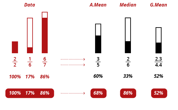
Underneath the three statistics, you will see both a black percentage, which is calculated from the average whole and average part, and a red percentage, which is an average of the ratios in the data. Only for the geometric mean are they the same.
For an information designer, this property is extremely useful because it means the final ratio can be graphed right along with the average whole and average part ? and there is no possible inconsistency.
Inconsistency could also be avoided with the arithmetic mean, but only by choosing the (black) ratio of averages. which has a particular meaning: it is a ratio that gives more weight to the items with higher values. In our example, the 6/7 counts for more than the 2/2. Now, this may be an interpretation you like, but it will depend on the situation. The average of ratios (red), on the other hand, treats each item equally (as does the geometric mean). This is desirable when only the ratio itself matters, not the size of the samples. Visually, you must choose whether to represent totals or ratios though ? unless you use the geometric mean.
Compound rates
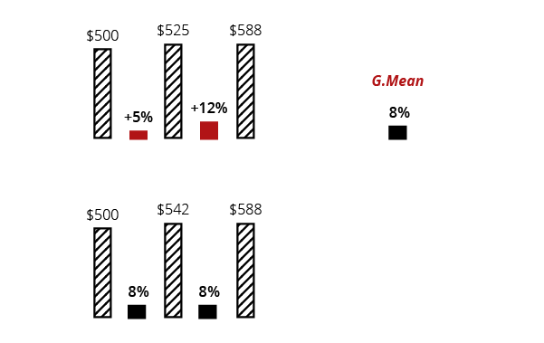
The main use of geometric means you?re likely to find described on the internet is calculating average compound interest, inflation, or investment returns. In these sorts of cases, you have a series of ratios that act multiplicatively: each one scales the previous total, in sequence. The geometric mean produces the most commonly sought-after summary here: the rate that all the rates would have to be if they were the same and produced the same final value.
Here?s an example with a $500 kitty that grows twice by a small percentage. If we replace the percentages with their geometric mean, the kitty grows to the same final value, $588.
Textbook problems are likely to call for a geometric mean. But it?s not impossible to need an arithmetic mean, like if you were trying to guess next year?s rate, or the median, if you want to split yearly rates into high and low categories. Again, there is no single master statistic that applies to a given type of data: it depends on what you?re looking for.
They?re Not Just for Money
Data that combine multiplicatively, like rates, are actually very common outside of economics too. The key is to recognize when a measured variables is affected by many (semi) independent forces, each of which scales that variable up or down ? rather than simply adding or subtracting a fixed amount to it. This is often true in the natural sciences.
For instance, soil conditions may be favorable to the growth of organisms, and Increasing Nitrogen content could improve biomass by 10%. But the exact numerical increase will dependent on many other environmental factors: you cannot assume a +10 ton increase, say, across all situations.
And More Common Than You Think
The way data are commonly presented may make them appear additive (arithmetic), when the underlying forces are in fact multiplicative (geometric). I think this happens when the data are familiar ? so we assume they?re simple ? and when the causes for those data are mysterious or complex.
For instance, if you download tuition numbers for public universities, these might seem like datapoints that are simply brute facts, each set by some administrator or state legislature. But the truth is that local wages, taxes, campus amenities, graduation rates, and the composition of the student body all play a role in making tuition what it is. And while the exact relationships may be diffuse and complex, we can bet they are indeed related as factors, not plus-or-minus changes. Therefore we should take a geometric mean of tuitions to find their central tendency.
Different Scales
The geometric mean is also excellent for constructing composite indices, utilizing very different sorts of data that are all scored differently. The reason is, the geometric mean is indifferent to the scales used (as long as the same ones are used each time).
For instance, you can combine a 570 SAT score with a 5/6 entrance essay, and 3 stars for sports, and 95% likelihood of paying tuition ? you don?t have to try normalizing the scores first. This doesn?t work with an arithmetic mean, where scores on the biggest scale (the SAT here) will dominate the average; basically you?d be weighting each value according to its scale.
Evenness
Evenness is how consistent or ?smooth? your data look, regardless of the bigger patterns in distribution or value; unneven data appear rough or noisy. As you may know, the arithmetic mean doesn?t measure evenness: all that matters is the total sum of value, and the number of items. The median also ignores roughness. Here?s an example to illustrate, with smooth (A) and noisy (B) data:
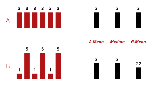
Only the geometric mean is sensitive to unevenness ? where it produces a lowered score. Being able to measure consistency can be useful: for instance, in public health, a single outbreak of bacteria in the drinking water is as bad, or worse, than many lower-level instances.
But there is a drawback. Imagine you calculate a geometric mean, get an unusually low score, and wonder why. There?s no way to tell if that reduction is caused by unevenness or just lower values across the board. If evenness will cause you interpretive headaches, or it really doesn?t matter, go with an arithmetic mean instead.
Logarithms
A convenient property of the geometric mean is that it?s equivalent to log-transforming your data, taking a regular arithmetic mean, and then transforming the result back (with the ?antilog? exponent). You can see that equivalence here:
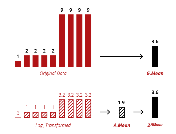
There?s no real reason to perform a geometric mean calculation with logarithms, but scientists often work with logged data anyway, and this property makes getting the geometric mean easy.
Beware Averages of Transformed Data
But the corollary is that you shouldn?t naively calculate averages on transformed data. You could inadvertently be taking an average of an average, with results that are difficult to interpret, and not what you expected. Theoretical ecologists spent years trying to understand a mysterious pattern in nature, only to finally realize it was an artifact of binning log-transformed data ? which had become a standard practice.
As an information designer, I don?t use use logarithmic transformation very often: it?s too hard for ordinary readers to understand a scale that isn?t regular. But one good use is turning percentages into ratios. For instance, by using the second logarithm, you can get ratios with the powers of 2 ? turning 0.5 and 0.25 into 2:1 and 4:1. Ratios are relatively familiar to most people (from sports and betting), and as with any logarithmic scale, this will spread out values at the low end of things, making them easier to see.
Removing Zeros
The geometric mean won?t be informative if zeros (or negatives) are present in the data. So one might be tempted to adjust them somehow so that it can work. This is probably a bad idea. But two circumstances might allow it, as far as I can see.
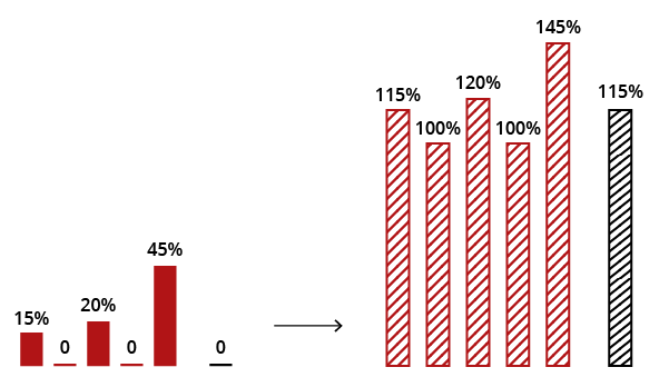
First, if you data can reasonably be interpreted as percentage increases, you can transform them into normal percentage values; e.g., +15% becomes 115%. Zeros then become 100%, and you can proceed with the calculation. You could then convert back to the original form by subtracting 100% if you wanted. But don?t do this simply out of convenience: the results have to be meaningful.
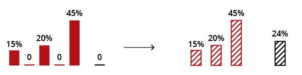
Second, if zeros can reasonably be interpreted as non-responses, which shouldn?t really count at all, they can be deleted. Again, though, the meaning of your summary statistics will change, from ?central tendency of the data? to ?central tendency of the responses.? Don?t trick yourself into doing this when it makes no sense . The results will also not be the same as in the first procedure either, as you can see.
Finally, I?ve also seen some people add the smallest value in their dataset to every value. This does allow the mean to be computed, which remains similar to the median. But one study found that the exact amount being added had a significant effect on certain results, which would make them very volatile and dependent on sampling. So I would avoid this, personally.
Some other Tidbits
There?s a strict ordering of the results you get from the arithmetic, geometric, and harmonic means. The geometric mean will always be smaller than the arithmetic, and the harmonic will be the smallest of all. The one exception is for perfectly uniform data, in which case they?re all the same. Where the median lies depends on the distribution of the data.
All three means are instances of the ?generalized mean.? It?s basically a generic algorithm that calls for raising the data to a certain power, adding the values together, dividing by the number of items, and then taking the root (the inverse of the power). The specific means vary in their power and root. The arithmetic mean uses a power of 1 (which does nothing, making the arithmetic mean just simple addition and division). The harmonic mean uses -1. And the geometric uses 0. The minimum and maximum can also be seen as generalized means, using powers of negative infinity and infinity.
Parting Thought
We don?t live in a world that?s simple, linear, or additive ? so don?t pretend we do when you do statistics and try to graph data. Sometimes the arithmetic mean will be useful, but don?t use it just because it?s familiar. The geometric mean has a lot of nice properties, as does the median. But there?s no master statistic to rule them all: you get a choice. Consider the data you have, how they?re related, and the questions you?re interested in; then pick tools that will help you make sense of those data and explain them to other people.

