 Photo by Nick Fewings on Unsplash
If you can?t explain it to a six year old, you don?t understand it yourself.
The world still awaits the next Einstein, or perhaps it won?t ever get another person of the century. But I like to believe: in the universe and in a variation of the above quote?
The best way to learn is to teach.
The idea for this post came when I was once helping one of my juniors with an assignment on outlier detection. It wasn?t a very complicated one, just an application of IQR Method of Outlier Detection on a dataset. The tutorial took an exciting turn when he asked me:
?Why 1.5 times IQR? Why not 1 or 2 or any other number??
Now this question won?t ring any bells for those who are not familier with IQR Method of Outlier Detection (explained below), but for those who know how simple this method is, I hope the question above would make you think about it. After all, isn?t that what good data scientists do? Question everything, believe nothing.
In the most general sense, an outlier is a data point which differs significantly from other observations. Now its meaning can be interpreted according to the statistical model under study, but for the sake of simplicity and not to divert too far from the main agenda of this post, we?d consider first order statistics and too on a very simple dataset, without any loss of generality.
IQR Method of Outlier Detection
To explain IQR Method easily, let?s start with a box plot.
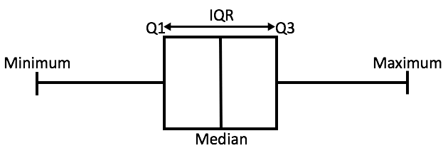 A box plot from source
A box plot tells us, more or less, about the distribution of the data. It gives a sense of how much the data is actually spread about, what?s its range, and about its skewness. As you might have noticed in the figure, that a box plot enables us to draw inference from it for an ordered data, i.e., it tells us about the various metrics of a data arranged in ascending order.
In the above figure,
- minimum is the minimum value in the dataset,
- and maximum is the maximum value in the dataset.
So the difference between the two tells us about the range of dataset.
- The median is the median (or centre point), also called second quartile, of the data (resulting from the fact that the data is ordered).
- Q1 is the first quartile of the data, i.e., to say 25% of the data lies between minimum and Q1.
- Q3 is the third quartile of the data, i.e., to say 75% of the data lies between minimum and Q3.
The difference between Q3 and Q1 is called the Inter-Quartile Range or IQR.
IQR = Q3 – Q1
To detect the outliers using this method, we define a new range, let?s call it decision range, and any data point lying outside this range is considered as outlier and is accordingly dealt with. The range is as given below:
Lower Bound: (Q1 – 1.5 * IQR)Upper Bound: (Q3 + 1.5 * IQR)
Any data point less than the Lower Bound or more than the Upper Bound is considered as an outlier.
But the question was: Why only 1.5 times the IQR? Why not any other number?
Well, as you might have guessed, the number (here 1.5, hereinafter scale) clearly controls the sensitivity of the range and hence the decision rule. A bigger scale would make the outlier(s) to be considered as data point(s) while a smaller one would make some of the data point(s) to be perceived as outlier(s). And we?re quite sure, none of these cases is desirable.
But this is an abstract way of explaining the reason, it?s quite effective, but naive nonetheless. So to what should we turn our heads for hope?
Maths! Of course! (You saw that coming, right? ?)
Things are gonna get a bit ?math-y? from here on after. But I?ll try to keep it minimal.
You might be surprised if I tell you that this number, or scale, depends on the distribution followed by the data.
For example, let?s say our data follows, our beloved, Gaussian Distribution.
Gaussian Distribution
You all must have seen how a Gaussian Distribution looks like, right? If not, here it is (although I?m suspicious about you ?).
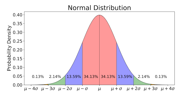 Gaussian Distribution with steps of standard deviation from source
There are certain observations which could be inferred from this figure:
- About 68.26% of the whole data lies within one standard deviation (<?) of the mean (?), taking both sides into account, the pink region in the figure.
- About 95.44% of the whole data lies within two standard deviations (2?) of the mean (?), taking both sides into account, the pink+blue region in the figure.
- About 99.72% of the whole data lies within three standard deviations (<3?) of the mean (?), taking both sides into account, the pink+blue+green region in the figure.
- And the rest 0.28% of the whole data lies outside three standard deviations (>3?) of the mean (?), taking both sides into account, the little red region in the figure. And this part of the data is considered as outliers.
- The first and the third quartiles, Q1 and Q3, lies at -0.675? and +0.675? from the mean, respectively.
I could have shown you the calculations behind these inferences but that?s beyond the scope of this article. If you wish, you can check these at: cs.uni.edu/~campbell/stat/normfact.html
Let?s calculate the IQR decision range in terms of ?
Taking scale = 1:
Lower Bound:= Q1 – 1 * IQR= Q1 – 1 * (Q3 – Q1)= -0.675? – 1 * (0.675 – [-0.675])?= -0.675? – 1 * 1.35?= -2.025?Upper Bound:= Q3 + 1 * IQR= Q3 + 1 * (Q3 – Q1)= 0.675? + 1 * (0.675 – [-0.675])?= 0.675? + 1 * 1.35?= 2.025?
So, when scale is taken as 1, then according to IQR Method any data which lies beyond 2.025? from the mean (?), on either side, shall be considered as outlier. But as we know, upto 3?, on either side of the ? ,the data is useful. So we cannot take scale = 1, because this makes the decision range too exclusive, means this results in too much outliers. In other words, the decision range gets so small (compared to 3?) that it considers some data points as outliers, which is not desirable.
Taking scale = 2:
Lower Bound:= Q1 – 2 * IQR= Q1 – 2 * (Q3 – Q1)= -0.675? – 2 * (0.675 – [-0.675])?= -0.675? – 2 * 1.35?= -3.375?Upper Bound:= Q3 + 2 * IQR= Q3 + 2 * (Q3 – Q1)= 0.675? + 2 * (0.675 – [-0.675])?= 0.675? + 2 * 1.35?= 3.375?
So, when scale is taken as 2, then according to IQR Method any data which lies beyond 3.375? from the mean (?), on either side, shall be considered as outlier. But as we know, upto 3?, on either side of the ? ,the data is useful. So we cannot take scale = 2, because this makes the decision range too inclusive, means this results in too few outliers. In other words, the decision range gets so big (compared to 3?) that it considers some outliers as data points, which is not desirable either.
Taking scale = 1.5:
Lower Bound:= Q1 – 1.5 * IQR= Q1 – 1.5 * (Q3 – Q1)= -0.675? – 1.5 * (0.675 – [-0.675])?= -0.675? – 1.5 * 1.35?= -2.7?Upper Bound:= Q3 + 1.5 * IQR= Q3 + 1.5 * (Q3 – Q1)= 0.675? + 1.5 * (0.675 – [-0.675])?= 0.675? + 1.5 * 1.35?= 2.7?
When scale is taken as 1.5, then according to IQR Method any data which lies beyond 2.7? from the mean (?), on either side, shall be considered as outlier. And this decision range is the closest to what Gaussian Distribution tells us, i.e., 3?. In other words, this makes the decision rule closest to what Gaussian Distribution considers for outlier detection, and this is exactly what we wanted.
*** Side Note ***
To get exactly 3?, we need to take the scale = 1.7, but then 1.5 is more ?symmetrical? than 1.7 and we?ve always been a little more inclined towards symmetry, aren?t we!?
Also, IQR Method of Outlier Detection is not the only and definitely not the best method for outlier detection, so a bit trade-off is legible and accepted.
See, how beautifully and elegantly it all unfolded using maths. I just love how things become clear and evidently takes shape when perceived through its mathematics. And this is one of the many reasons why maths is the language of our world (not sure about the universe though ?).
So, I hope, now you know why do we take it 1.5 * IQR. But this scale depends on the distribution followed by the data. Say if my data seem to follow exponential distribution then this scale would change.
But again, every complication which arises because of mathematics is solved by mathematics itself.
Ever heard of Central Limit Theorem? Yep! The very same theorem why grants us the liberty to assume the distribution to be followed as Gaussian without any guilt. But I think I?d leave that for some other day. Until then, be curious!
Hope you found this article useful. Thanks!
Godspeed!

