Whenever working on a data set to predict or classify a problem, we tend to find accuracy by implementing a design model on first train set, then on test set. If the accuracy is satisfactory, we tend to increase accuracy of data-sets prediction either by increasing or decreasing data feature or features selection or applying feature engineering in our machine learning model. But sometime our model maybe giving poor result.
The poor performance of our model maybe because, the model is too simple to describe the target, or may be model is too complex to express the target. Why this happened? And how to deal with it?
Why Our model perform poor sometime?
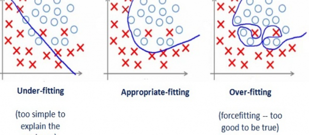
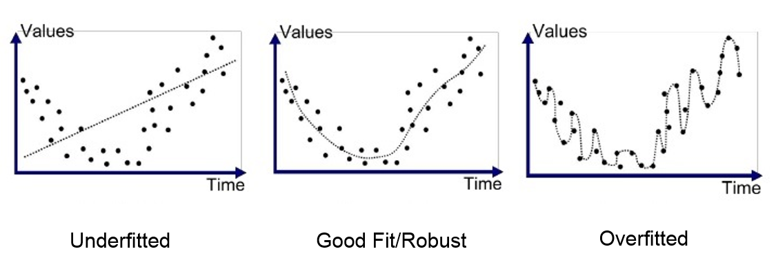
So here comes the concept of overfitting and underfitting. Overfitting and underfitting can be explained using below graph.
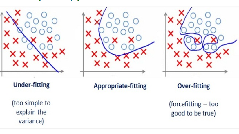
By looking at the graph on the left side we can predict that the line does not cover all the points shown in the graph. Such model tend to cause underfitting of data .It also called High Bias.
Where as the graph on right side, shows the predicted line covers all the points in graph. In such condition you can also think that it?s a good graph which cover all the points. But that?s not actually true, the predicted line into the graph covers all points which are noise and outlier. Such model are also responsible to predict poor result due to its complexity.It is also called High Variance.
Now, Looking at the middle graph it shows a pretty good predicted line. It covers majority of the point in graph and also maintains the balance between bias and variance.
In machine learning, we predict and classify our data in more generalized way. So in order to solve the problem of our model that is overfitting and underfitting we have to generalize our model. Statistical speaking how well our model fit to data set such that it gives proper accurate results as expected.
Now the question comes, How to differentiate between overfitting and underfitting?
Solving the issue of bias and variance is really about dealing with over-fitting and under-fitting. Bias is reduced and variance is increased in relation to model complexity. As more and more parameters are added to a model, the complexity of the model rises and variance becomes our primary concern while bias steadily falls.
Lets first learn what is bias, variance and their importance in predicting model.
Bias:It gives us how closeness is our predictive model?s to training data after averaging predict value. Generally algorithm has high bias which help them to learn fast and easy to understand but are less flexible. That looses it ability to predict complex problem, so it fails to explain the algorithm bias. This results in underfitting of our model.
Getting more training data will not help much.
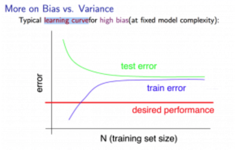
Variance:It define as deviation of predictions, in simple it is the amount which tell us when its point data value change or a different data is use how much the predicted value will be affected for same model or for different model respectively. Ideally, the predicted value which we predict from model should remain same even changing from one training data-sets to another, but if the model has high variance then model predict value are affect by value of data-sets.
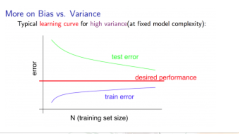
The Graph below shows the path when a learning algorithm suffers from High Variance. This show getting more training data will help to deal with it.
How to overcome it? And what are the techniques?
The method to overcome this overfitting and underfitting problem we have to see them separately one by one.
1 .Underfitting:
In order to overcome underfitting we have to model the expected value of target variable as nth degree polynomial yeilding the general Polynomial.The training error will tend to decrease as we increase the degree d of the polynomial.
The mathematical presentation can be give as,


The training error will tend to decrease as we increase the degree d of the polynomial.
At the same time, the cross validation error will tend to decrease as we increase d up to a point, and then it will increase as d is increased, forming a convex curve.
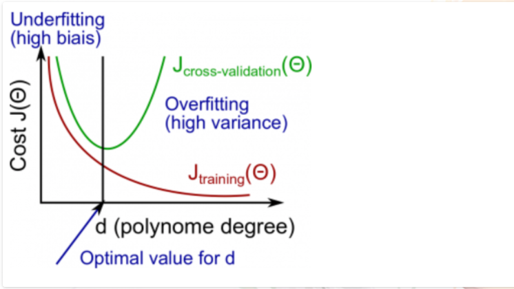
This concept of implementing this model is said Polynomial Regression, to get insight of Polynomial Regression click here.
Polynomial projection is built into scikit-learn using the polynomial feature transform.
2. Overfitting:
To solve the problem of overfitting inour model we need to increase flexibility of our model. But too much of his flexibility can also spoil our model, so flexibility shold such that it is optimal value. To increase flexibility we can use regularization technique.
They are three types of regularization technique to overcome overfitting.
a) L1 regularization (also called Lasso regularization / panelization.)
b) L2 regularization (also called Ridege regularization/ penalization.)
c) Elastic net
Let?s see detailed explanation of each one by one.
a) L1 regularization:
It stand for? least absolute shrinkage and and selection operator?.
Mathematical representation of it can be given as,
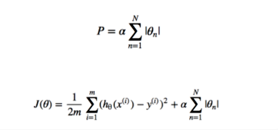
Things we need to reduce the overfitting of data, the ?P? term should be added to our existing model and alpha is learning rate. Lasso method overcome the disadvantage of Ridge regression by not furnishing high value of the coefficient beta but actually setting them to 0 you they are not relavent, therefore you might end with fewer features including the model you started with, which is the huge advantage.
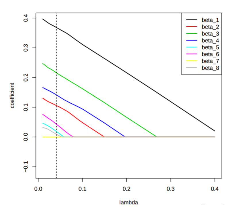
Limitation of Lasso:
i) If p>n, the lasso selects at most n variables. The number of selected genes is bounded by the number of samples. Where ?p? is number of data and ?n? are train and test samples.
ii) Grouped variables: the lasso fails to do grouped selection. It tends to select one variable from a group and ignore the others.
To get more insight of L1 regulation(Lasso regression) click here.
b) l2 regularization:
It is also known as ?Tikhnov regularization?.
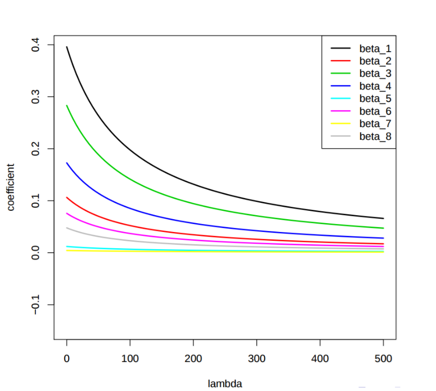
Mathematical it is given as,

The ?P? is the regularization added to cost function.The importance of this regularization is such that it enforces the Beta function to be lower, but it does not enforces then to zero. That is that is it will not get rid of features which are not suitable but rather minimize the impact on the trained model.
3. Elastic:
Working of Elastic regularization is such that it work by implementing both i.e Lasso and Ridge together. Hence, it work more better then both individual.
The elastic net solution path is piece wise linear. The mathematical representation is given as,

The advantage of Elastic regularization is that it overcome limitation of both Lasso and Ridge to some extend.
Conclusion:
Applying machine learning model on data-sets directly, will not predict our accuracy as we expected and it may be full of overfitting or underfitting representation on our training data. This blog shows short intro on overfitting and underfitting, identifying and how to solve when it occur using regularization technique. To see proper intuition of applying regularization technique working and how much our accuracy score differ before and after applying on Iris-data .
Though the above link show how we can increase our accuracy just using regularization and dealing with overfitting and underfitting, but there is also equal important that we should do proper study of our datasets, before even starting our project. Hopefully you learn overfitting , underfitting, identifying, dealing with it using regularization. Data science is field which has lots to learn and also to contribute to world. The only challenges is one should have willing to learn more and give it back society.
