What are Eigenvalues and Eigenvectors?

A must-know concept for Machine Learning

Eigenvectors and eigenvalues live in the heart of the data science field. This article will aim to explain what eigenvectors and eigenvalues are, how they are calculated and how we can use them. It?s a must-know topic for anyone who wants to understand machine learning in-depth.

Eigenvalues and eigenvectors form the basics of computing and mathematics. They are heavily used by scientists.

Article Structure

This article is structured in six parts:

1. I will start by providing a brief introduction of eigenvectors and eigenvalues.
2. Then I will illustrate their use-cases and applications.
3. I will then explain the building blocks that make up the eigenvalues and eigenvectors such as the basics of matrix addition and multiplication so that we can refresh our knowledge and understand the concepts thoroughly.
4. I will then illustrate how eigenvectors and eigenvalues are calculated.
5. Subsequently, a working example of how eigenvectors and eigenvalues are calculated will be presented.
6. Finally, I will outline how we can compute the eigenvectors and eigenvalues in Python.

1. Eigenvectors and Eigenvalues Introduction

Before we take a deep dive into calculating eigenvectors and eigenvalues, let?s understand what they really are.

Let?s consider that we want to build mathematical models (equations) where the input data is gathered from a large number of sources. As an instance, let?s assume that we want to forecast a complex financial variable, such as the behavior of interest rates over time. Let?s refer to interest rates as y.

The first step might involve finding the variables that y is dependent on. Let?s refer to these variables as x(i)

We will start our research by gathering data for variables that y is dependent on. Some of the data might be in textual format. The task would be to convert the non-numerical data into numerical data. As an instance, we often use one-hot encoding to transform values in textual features to separate numerical columns. If our input data is in images format then we would have to somehow convert the image into numerical matrices.

The second step would be to join the data into a tabular format where each column of the table is computed by 1 or more features. This will result in a large sparse matrix (table). At times, it can increase our dimension space to 100+ columns.

Now let?s understand this!

It introduces its own sets of problems such as the large sparse matrix can end up taking a significant amount of space on a disk. Plus, it becomes extremely time-consuming for the model to train itself on the data. Furthermore, it is difficult to understand and visualize data with more than 3 dimensions, let alone a dataset of over 100+ dimensions. Hence, it would be ideal to somehow compress/transform this data into a smaller dataset.

There is a solution. We can utilise Eigenvalues and Eigenvectors to reduce the dimension space. To elaborate, one of the key methodologies to improve efficiency in computationally intensive tasks is to reduce the dimensions after ensuring most of the key information is maintained.

Eigenvalues and Eigenvectors are the key tools to use in those scenarios

1.1 What Is An Eigenvector?

I would like to explain this concept in a way that we can easily understand it.

For the sake of simplicity, let?s consider that we live in a two-dimensional world.

• Alex?s house is located at coordinates [10,10] (x=10 and y =10). Let?s refer to it as vector A.
• Furthermore, his friend Bob lives in a house with coordinates [20,20] (x=20 and y=20). I will refer to it as vector B.

If Alex wants to meet Bob at his place then Alex would have to travel +10 points on the x-axis and +10 points on the y-axis. This movement and direction can be represented as a two-dimensional vector [10,10]. Let?s refer to it as vector C.

We can see that vector A to B are related because vector B can be achieved by scaling (multiplying) the vector A by 2. This is because 2 x [10,10] = [20,20]. This is the address of Bob. Vector C also represents the movement for A to reach B.

The key to note is that a vector can contain the magnitude and direction of a movement. So far so good!

We learned from the introduction above that large set of data can be represented as a matrix and we need to somehow compress the columns of the sparse matrix to speed up our calculations. Plus if we multiply a matrix by a vector then we achieve a new vector. The multiplication of a matrix by a vector is known as transformation matrices.

We can transform and change matrices into new vectors by multiplying a matrix with a vector. The multiplication of the matrix by a vector computes a new vector. This is the transformed vector. Hold that thought for now!

The new vector can be considered to be in two forms:

1. Sometimes, the new transformed vector is just a scaled form of the original vector. This means that the new vector can be re-calculated by simply multiplying a scalar (number) to the original vector; just as in the example of vector A and B above.
2. And other times, the transformed vector has no direct scalar relationship with the original vector which we used to multiply to the matrix.

If the new transformed vector is just a scaled form of the original vector then the original vector is known to be an eigenvector of the original matrix. Vectors that have this characteristic are special vectors and they are known as eigenvectors. Eigenvectors can be used to represent a large dimensional matrix.

Therefore, if our input is a large sparse matrix M then we can find a vector o that can replace the matrix M. The criteria is that the product of matrix M and vector o should be the product of vector o and a scalar n:

M * o = n* o

This means that a matrix M and a vector o can be replaced by a scalar n and a vector o.

In this instance, o is the eigenvector and n is the eigenvalue and our target is to find o and n.

Therefore an eigenvector is a vector that does not change when a transformation is applied to it, except that it becomes a scaled version of the original vector.

Eigenvectors can help us calculating an approximation of a large matrix as a smaller vector. There are many other uses which I will explain later on in the article.

Eigenvectors are used to make linear transformation understandable. Think of eigenvectors as stretching/compressing an X-Y line chart without changing their direction.

1.2 What is an Eigenvalue?

Eigenvalue??The scalar that is used to transform (stretch) an Eigenvector.

Let?s understand where eigenvalues and eigenvectors are used

2. Where are Eigenvectors and Eigenvalues used?

There are multiple uses of eigenvalues and eigenvectors:

1. Eigenvalues and Eigenvectors have their importance in linear differential equations where you want to find a rate of change or when you want to maintain relationships between two variables.

Think of eigenvalues and eigenvectors as providing summary of a large matrix

2. We can represent a large set of information in a matrix. Performing computations on a large matrix is a very slow process. To elaborate, one of the key methodologies to improve efficiency in computationally intensive tasks is to reduce the dimensions after ensuring most of the key information is maintained. Hence, one eigenvalue and eigenvector are used to capture key information that is stored in a large matrix. This technique can also be used to improve the performance of data churning components.

3. Component analysis is one of the key strategies that is utilised to reduce dimension space without losing valuable information. The core of component analysis (PCA) is built on the concept of eigenvalues and eigenvectors. The concept revolves around computing eigenvectors and eigenvalues of the covariance matrix of the features.

4. Additionally, eigenvectors and eigenvalues are used in facial recognition techniques such as EigenFaces.

5. They are used to reduce dimension space. The technique of Eigenvectors and Eigenvalues are used to compress the data. As mentioned above, many algorithms such as PCA rely on eigenvalues and eigenvectors to reduce the dimensions.

6. Eigenvalues are also used in regularisation and they can be used to prevent overfitting.

Eigenvectors and eigenvalues are used to reduce noise in data. They can help us improve efficiency in computationally intensive tasks. They also eliminate features that have a strong correlation between them and also help in reducing over-fitting.

6. Occasionally we gather data that contains a large amount of noise. Finding important or meaningful patterns within the data can be extremely difficult. Eigenvectors and eigenvalues can be used to construct spectral clustering. They are also used in singular value decomposition.

7. We can also use eigenvector to rank items in a dataset. They are heavily used in search engines and calculus.

8. Lastly, in non-linear motion dynamics, eigenvalues and eigenvectors can be used to help us understand the data better as they can be used to transform and represent data into manageable sets.

Having said that, it can be slow to compute eigenvectors and eigenvalues. The computation is O(n)

Photo by Helloquence on Unsplash

It is now apparent that Eigenvalues and Eigenvectors are one of core concepts to understand in data science. Hence this article is dedicated to them.

Have a look at this article if you want to understand dimension reduction and PCA:

What Is Dimension Reduction In Data Science?

We have access to a large amounts of data now. The large amount of data can lead us to create a forecasting model where?

medium.com

Photo by Joel Filipe on Unsplash

3. What are the building blocks of Eigenvalues and Eigenvectors?

Let?s understand the foundations of Eigenvalues and Eigenvectors.

Eigenvectors and eigenvalues revolve around the concept of matrices.

Matrices are used in machine learning problems to represent a large set of information. Eigenvalues and eigenvectors are all about constructing one vector with one value to represent a large matrix. Sounds very useful, right?

What is a matrix?

• A matrix has a size of X rows and Y columns, like a table.
• A square matrix is the one that has a size of n, implying that X and Y are equal.
• A square matrix is represented as A. This is an example of a square matrix

Let?s quickly recap and refresh how matrix multiplication and addition works before we take a deep dive

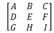
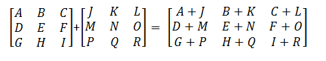
3.1 Matrix Addition

Matrix addition is simply achieved by taking each element of a matrix and adding it together as shown below:

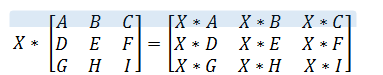
3.2 Multiplying Scalar With A Matrix

Multiplying Matrix by a scalar is as straight forward as multiplying each element by the scalar:

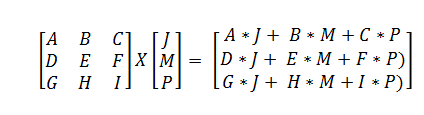
3.3 Matrices Multiplication

Matrices multiplication is achieved by multiplying and then summing matching members of the two matrices. The image below illustrates how we can multiple a 3 by 3 and a 3 by 1 matrix together:

That?s all the Maths which we need to know for the moment

4. Calculating Eigenvectors and Eigenvalues

Although we don?t have to calculate the Eigenvalues and Eigenvectors by hand every time but it is important to understand the inner workings to be able to confidently use the algorithms.

4.1 Let?s understand the steps first

Key Concepts: Let?s go over the following bullet points before we calculate Eigenvalues and Eigenvectors

Eigenvalues and Eigenvectors have following components:

• The eigenvector is an array with n entries where n is the number of rows (or columns) of a square matrix. The eigenvector is represented as x.
• Key Note: The direction of an eigenvector does not change when a linear transformation is applied to it.
• Therefore, Eigenvector should be a non-null vector
• We are required to find a number of values, known as eigenvalues such that

A * x = lambda * x

The above equation states that we need to find eigenvalue (lambda) and eigenvector (x) such that when we multiply a scalar lambda (eigenvalue) to the vector x (eigenvector) then it should equal to the linear transformation of the matrix A once it is scaled by vector x (eigenvector).

Eigenvalues are represented as lambda.

Keynote: The above equation should not be invertible.

There are two special keywords which we need to understand: Determinant of a matrix and an identity matrix

• The determinant of a matrix is a number that is computed from a square matrix. In a nutshell, the diagonal elements are multiplied by each other and then they are subtracted together. We need to ensure that the determinant of the matrix is 0.
• Last component: We need an Identity Matrix. An identity square matrix is a matrix that has 1 in diagonal and all of its elements are 0. The identity matrix is represented as I:

We can represent

A * x = lambda * xAs:A * x – lambda * x = 0

Now, we need to compute a characteristic equation.

|A – Lambda * I| = 0

Subsequently

Determinant(A – Lambda * I) = 0

4.2 How do I calculate Eigenvalue?

The task is to find Eigenvalues of size n for a matrix A of size n.

Therefore, the aim is to find: Eigenvector and Eigenvalues of A such that:

A * Eigenvector ? Eigenvalue * EigenVector = 0

Find Lambda Such that Determinant(A ? Lambda * I) = 0

Based on the concepts learned above:

1. lambda * I is:

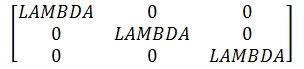
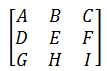
If A is:

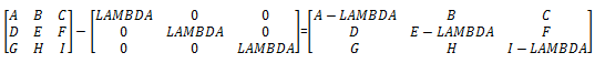
2. Then A ? lambda * I is:

3. Finally calculate the determinant of (A-lambda*I) as:

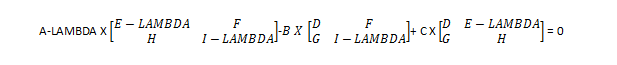
Once we solve the equation above, we will get the values of lambda. These values are the Eigenvalues.

I will present a working example below to illustrate the theory so that we understand the concepts thoroughly.

4.3 How do I calculate Eigenvector?

Once we have calculated eigenvalues, we can calculate the Eigenvectors of matrix A by using Gaussian Elimination. Gaussian elimination is about converting the matrix to row echelon form. Finally, it is about solving the linear system by back substitution.

A detailed explanation of Gaussian elimination is out of the scope of this article so that we can concentrate on Eigenvalues and Eigenvectors.

Once we have the Eigenvalues, we can find Eigenvector for each of the Eigenvalues. We can substitute the eigenvalue in the lambda and we will achieve an eigenvector.

(A – lambda * I) * x = 0

Therefore if a square matrix has a size n then we will get n eigenvalues and as a result, n eigenvectors will be computed to represent the matrix.

Now that we have the key, it is the time to compute the Eigenvalues and Eigenvectors together.

Photo by CMDR Shane on Unsplash

5. Practical Example: Let?s calculate Eigenvalue and Eigenvector together

If there are any doubts then do inform me.

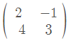
Let?s find eigenvalue of the following matrix:

First, multiply lambda to an identity matrix and then subtract the two matrices

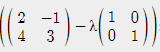
We need to compute a determinant of:

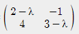
Therefore:

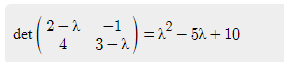
Once we solve the quadratic equation above, we will yield two Eigenvalues:

Now that we have computed Eigenvalues, let?s calculate Eigenvectors together

Take the first Eigenvalue (Lambda) and substitute the eigenvalue into the following equation:

(A – lambda * I)

For the first eigenvalue, we will get the following Eigenvector:

Plug-in to get the matrix

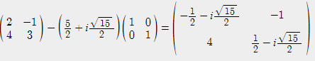
Gives:

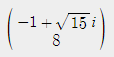
This Eigenvector now represents the key information of matrix A

I want you to find the second Eigenvector.

Message me your values and workings.

6. Calculate Eigenvalues and Eigenvectors in Python

Although we don?t have to calculate the Eigenvalues and Eigenvectors by hand but it is important to understand the inner workings to be able to confidently use the algorithms. Furthermore, It is very straightforward to calculate eigenvalues and eigenvectors in Python.

We can use numpy.linalg.eig module. It takes in a square matrix as the input and returns eigenvalues and eigenvectors. It also raises an LinAlgError if the eigenvalue computation does not converge.

import numpy as npfrom numpy import linalg as LAinput = np.array([[2,-1],[4,3]])w, v = LA.eig(input)print(w)print(v)

Summary

This article explained one of the key areas of machine learning. It started by giving a brief introduction of eigenvectors and eigenvalues.

Then it explained how eigenvectors and eigenvalues are calculated from the foundations of matrix addition and multiplication so that we can understand the key components thoroughly.

It then presented a working example. Lastly, it outlined how we can compute the eigenvectors and eigenvalues in Python.

I hope it helps. Please let me know if you have any questions or feedback.