
 Photo by Sbastien Marchand on Unsplash
There are two fundamental ways of graph search, which are the breadth-first search (BFS) and the depth-first search (DFS). In this post, I?ll explain the depth-first search. Here, I focus on the relation between the depth-first search and a topological sort. A topological sort is deeply related to dynamic programming which you should know when you tackle competitive programming. For its implementation, I used Python. If you?d like to know the breadth-first search, check my other post: Understanding the Breadth-First Search with Python.
1. The algorithm of the depth-first search
In the depth-first search, we visit vertices until we reach the dead-end in which we cannot find any not visited vertex. When we reach the dead-end, we step back one vertex and visit the other vertex if it exists. I?ll show the actual algorithm below.
1. Apply step 2 to the starting vertex2. Re-apply step 2 to the neighbor of the given vertex if the vertex is not visited
Step 2 is the most important step in the depth-first search. Basically, it repeatedly visits the neighbor of the given vertex. Note that it visits the not visited vertex. This is because the program has never ended when re-visiting.
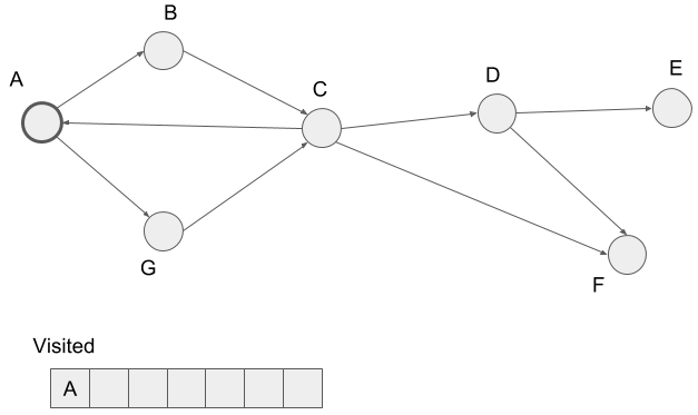
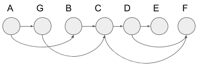
Let?s check the way how that algorithm works. On the figure below, we start the depth-first search from vertex A. Initial state will become as follows.
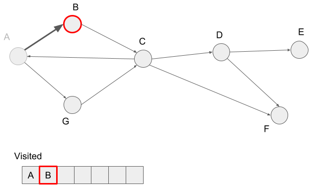
First, we visit vertex B, the neighbor of vertex A, and mark B visited. Note that we visit vertices in alphabetical order if the visiting vertex has multiple neighbors. So we don?t visit vertex G here.
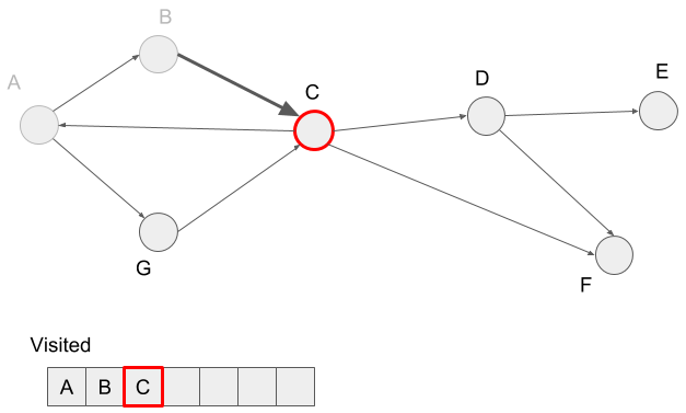
Then we visit the neighbor of vertex B, vertex C, and mark it visited.
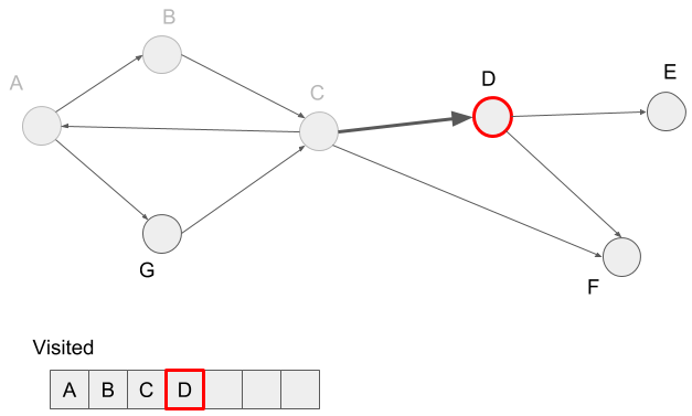
We try to visit the vertex C?s neighbor A, but it?s already visited. So we visit vertex D and mark it visited.
We visit the neighbor of vertex D, vertex E and mark vertex E visited.
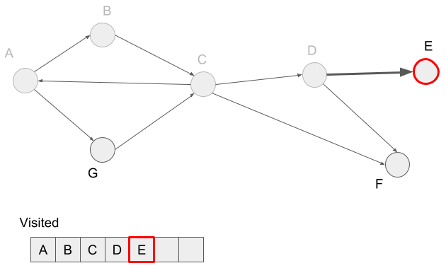
Vertex E doesn?t have neighbors, so we reached a dead-end. In the depth-first search, we visit the not visited neighbors of the visited vertex before reaching a dead-end. In this case, we visited vertex D before reaching the dead-end, so we visit the not visited neighbor F of the vertex D.
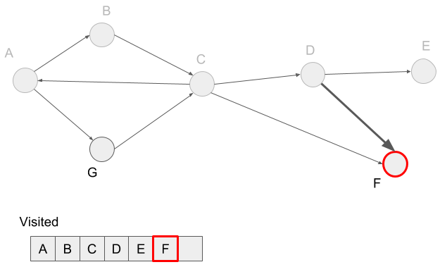
In the depth-first search, we first visit the vertices in one path and its neighbors, then visit vertices in another path. For example, A -> B and A -> G are two paths. We first visit all vertices in the first path, A -> B -> C -> D -> E -> F. And then visit the second path A -> G. We?ve already visited A, so just add G to the visited hash-table.
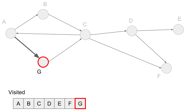
Here we visited all the vertices, so we get the depth-first search done.
2. Edge classification in the depth-first search
We get the path as a tree structure by the depth-first search as follows. We can get the following path when we apply the depth-first search to the graph used in the last section.
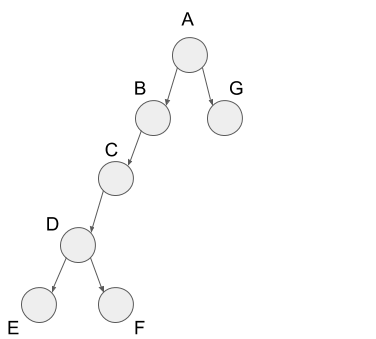
From the figure above, we got the characteristic tree structure. In the depth-first search, we classify the edges into four kinds below.
- tree edge
- forward edge
- back edge
- cross edge
I?ll describe these edges in details.
Tree edges are the edges included in the path of the depth-first search. So all the edges in the earlier figure are tree edges
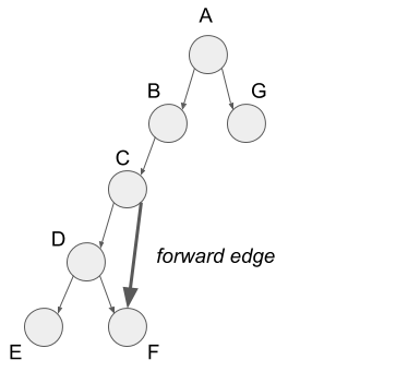
Rest of three edges are the edges not included in the path of the depth-first search but contained in the graph. First, forward edge is the edge from vertex C to vertex F. In the tree structure of the depth-first search, this edge goes from some node to the descendant node, so we call it the forward edge.
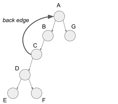
Next, I?ll explain back edges. The back edge is the edge from vertex C to vertex A. In the tree structure of the depth-first search, this edge goes from some node to the parent node, so we call it the back edge.
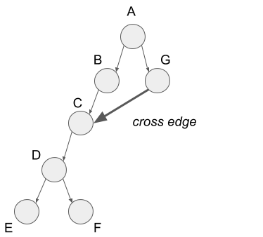
Finally, I?ll explain cross edges. The cross edge is the edge from vertex G to vertex C. In the tree structure of the depth-first search, this edge goes from some node in a sub-tree to the other node in other sub-tree, so we call it the cross edge.
That?s all for edge classification.
3. Relation to a topological sort
Here I?ll explain the relationship between the depth-first search and a topological sort. First, I?ll describe a topological sort and then explain the relation.
In a topological sort, we sort the vertices to make all edges go from left to right. Look at the graph below.
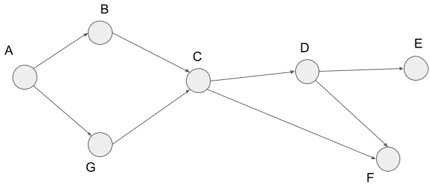
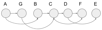
We get the figure below when we apply a topological sort to this graph. I?ll describe the way how to apply later. Also, I show the edges of the original graph above in the figure below. From the figure below, you can see all the edges go from left to right.
We call the node order above topological order. Let?s think what it tells us. Assume each vertex to be cooking steps for curry. Broadly speaking, the steps consist of cutting ingredients, seasoning meat, stir-frying them, and stewing. Here cutting ingredients or seasoning meat correspond to the vertices towards the left and stir-frying or stewing correspond to the vertices towards the right. This is because we cannot stew before cutting ingredients. So we can sort vertices in dependency order by using a topological sort. In the figure above, we put less dependent vertices from left to right.
On the other hand, we cannot use a topological sort to the following graph or the graph which has the part of the structure below. This is because all the vertices depend on the other vertices.
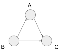
We call the path going around the vertices like this cycle. So we cannot use a topological sort to the graph has a cycle. We call the graph without any cycle directed acyclic graph, also known as DAG. The important thing is that if the graph can be topological-sorted, it is a DAG and DAG can be topological sorted.
We can get a topological order by applying the depth-first search to DAG. Look at the following DAG. This graph is the same as the example of a topological sort.
We can show the path of the depth-first search on this graph as this following tree structure.
We put each node in the tree structure from left to right by the order last visited in the depth-first search:

Then we reverse the order and add the edges in the original graph. We get the following figure. You can see this is a topological order.
Now we know we can get a topological order by applying the depth-first search to a DAG.
4. Implementation
We can implement the depth-first search with Python as follows.
def dfs(graph, vertex): parents = {vertex: None} dfs_visit(graph, vertex, parents)def dfs_visit(graph, vertex, parents): for n in graph[vertex]: if n not in parents: parents[n] = vertex dfs_visit(graph, n, parents)
We?re initializing to start the depth-first search in this line.
parents = {vertext: None}
We manage the vertices if they are visited by using keys in the parents. Also, values in parents correspond to the visited vertices before visiting the vertex of the key in parents. We call this variable ?parents? because it manages the parent node in the tree structure of the depth-first search. It means parents[key] returns the parent node (some vertex in a graph) of the key node (also another vertex in a graph).
dfs_visit is the main process of the depth-first search.
def dfs_visit(graph, vertex, parents): for n in graph[vertex]: if n not in parents parents[n] = vertex dfs_visit(graph, n, parents)
In this operation, we extract the neighbors of the given vertex and apply dfs_visit to the extracted vertex if it?s not marked visited. Note that graph[vertex] returns the neighbors of the vertex. When the recursively called dfs_visit is done, it gets back to the for-loop and applies the same operation to the other neighbors. After the first for-loop is finished, we can reconstruct the path of the depth-first search from parents.
Let?s think about the time complexity of the depth-first search. Its time complexity will be the called number of dfs_visit because the other operations take constant time. We call dfs_visit in the number of neighbors of the vertex times inside dfs_visit. In other words, we call dfs_visit in the number of degree of the vertex inside dfs_visit. In the worst case, we should call dfs_visit in the number of all the vertices times. So the time complexity will be the sum of the number of all the vertices and the number of the degrees of each vertex. The number of the degrees of each vertex will become 2|E| by the handshaking lemma. Therefore, the depth-first search run in O(|V|+|E|). Note that V is a set of vertices and E is a set of edges. I explain the handshaking lemma in my other post: Understanding the Breadth-First Search with Python. So if you are not familiar with it, please check it out.
That?s all for the explanation for the relationship between the depth-first search and the topological sort. Topological order deeply relates to dynamic programming. So I recommend you to keep it in mind if you?re going to tackle competitive programming. Thank you for reading.
References
- MIT OpenCourseWare 6.006 Lecture 14: Depth-First Search (DFS), Topological Sort
- MIT OpenCourseWare 6.006 Recitation 14: Depth-First Search (DFS)
