Please note that this post is for my future self to look back and review the materials on this paper without reading it all over again?.
In this blog i am trying to give a brief overview of Receptive Field in CNN and the mathematical calculation behind it .
To understand this post, I assume that you are familiar with the CNN concept, especially the convolutional and pooling operations. You can refresh your CNN knowledge by going through the paper ?A guide to convolution arithmetic for deep learning [1]?. It will not take you more than half an hour if you have some prior knowledge about CNNs.
All of the state-of-the-art object recognition methods design their model architectures around this idea.The receptive field is perhaps one of the most important concepts in Convolutional Neural Networks (CNNs) that deserves more attention from the literature.
1.Receptive Field and Feature map visualization
The receptive field can be briefly defined as the region in the input space that a particular CNN?s feature is looking at .A receptive field of a feature can be described by its center location and its size.However, not all pixels in a receptive field is equally important to its corresponding CNN?s feature.Within a receptive field, the closer a pixel to the center of the field, the more it contributes to the calculation of the output feature. Which means that a feature does not only look at a particular region in the input image, but also focus exponentially more to the middle of that region.
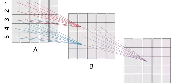
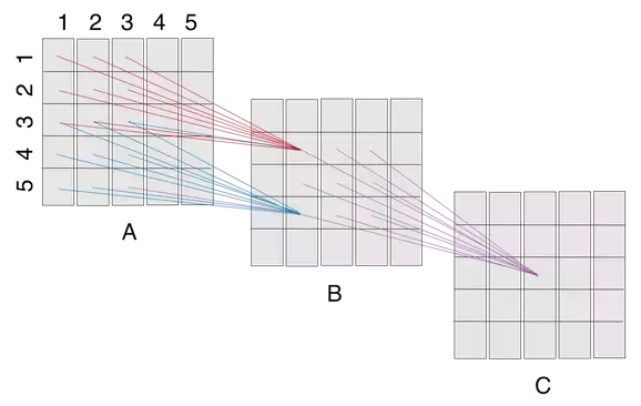 Fig1. CNN layer Visualization
Let us consider the above figure A, B and C would be convolutional layers of a CNN. (Padding not shown, but is required to maintain the same layer dimensions. Also, the stride is 1.) The filter size here is 3×3.The ?receptive field? of a ?neuron? in a layer would be the cross section of the previous layer from which neurons provide inputs. So, the receptive field of B(2,2) is the square A(1:3,1:3), that of B(4,2) is the square A(3:5,1:3), that of C(3,3) is B(2:4,2:4), and so on..Now the receptive field of C(3,3) is B(2:4,2:4), which itself receives inputs from A(1:5,1:5). So, rather than using a single filter of size 5, stacking 2 convolutional layers (without pooling) with 3×3 filters results in a net 5×5 filter. 3 such layers would give you an effective size of 7×7.
2.Calculating the size of a particular receptive field
For convolutional neural network, the number of output features in each dimension can be calculated by the following formula:. The number of output features in each dimension can be calculated using the following formula, which is explained in detail in [1].
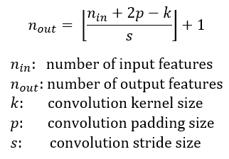 Fig2. Receptive Formula
I assume the CNN architecture to be symmetric, and the input image to be square. So both dimensions have the same values for all variables. If the CNN architecture or the input image is asymmetric, you can calculate the feature map attributes separately for each dimension.
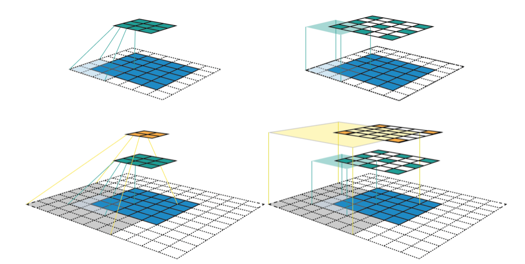 Fig3. CNN Feature map Visualization
For the upper left sub-figure, the input image is a 5 x 5 matrix (blue grid). Then zero-padding with size of p = 1 (transparent grid around the input image) is used to maintain the edge information during convolution. After that, a 3 x 3 kernel with stride of s = 2 is used to convolve this image to gain itsfeature map (green grid) with size of 3 x 3. In this example, nine features are obtained and each feature has a receptive field with size of 3 x 3 (the area inside light blue lines). We can use the same convolution on this green grid to gain a deeper feature map (orange grid) as shown in sub-figure at the left bottom. As for orange feature map, each feature has a 7 x 7 receptive field.
But if we only look at the feature map (green or orange grid), we cannot directly know which pixels a feature is looking at and how big is that region. The two sub-figures in the right column present another way to visualize the feature map, where the size of each feature map is fixed and equals to the size of input, and each feature is located at the center of its receptive field. In this situation, the only task is to calculate the area of the receptive field mathematically.
3.Receptive Field Arithmetic
To calculate the receptive field in each layer, besides the number of features nin each dimension, we need to keep track of some extra information for each layer. These include the current receptive field size r , the distance between two adjacent features (or jump) j, and the center coordinate of the upper left feature (the first feature) start. Note that the center coordinate of a feature is defined to be the center coordinate of its receptive field, as shown in the fixed-sized CNN feature map above. When applying a convolution with the kernel size k, the padding size p, and the stride size s, the attributes of the output layer can be calculated by the following equations:
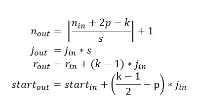 Fig4. Receptive field formula
- The first equation calculates the number of output features based on the number of input features and the convolution properties. This is the same equation presented in [1].
- The second equation calculates the jump in the output feature map, which is equal to the jump in the input map times the number of input features that you jump over when applying the convolution (the stride size).
- The third equation calculates the receptive field size of the output feature map, which is equal to the area that covered by k input features (k-1)*j_inplus the extra area that covered by the receptive field of the input feature that on the border.
- The fourth equation calculates the center position of the receptive field of the first output feature, which is equal to the center position of the first input feature plus the distance from the location of the first input feature to the center of the first convolution (k-1)/2*j_in minus the padding spacep*j_in. Note that we need to multiply with the jump of the input feature map in both cases to get the actual distance/space.
The first layer is the input layer, which always has n = image size, r = 1, j = 1, and start = 0.5. Note that in the Fig5 the coordinate system in which the center of the first feature of the input layer is at 0.5. By applying the four above equations recursively, we can calculate the receptive field information for all feature maps in a CNN. Fig5 shows an example of how these equations work.
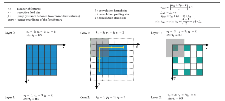
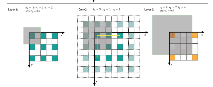 Fig5. Receptive field calculations on the Fig3
All these works aim at visualizing what convolutional neural networks learn. Besides the visualization of receptive fields, the visualization of Activation-Layers or visualization of filters/weights is also good ways to understand hidden layers in deep CNNs as shown in following figures (source: http://cs231n.github.io/understanding-cnn/):
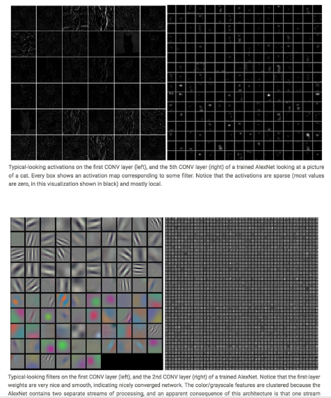 Fig6. CNN all layers visualization
Since I might not be an expert on the topic, if you find any mistakes in the article, or have any suggestions for improvement, please mention in comments.
References
https://medium.com/mlreview/a-guide-to-receptive-field-arithmetic-for-convolutional-neural-networks-e0f514068807

