Download IPython Notebook here.
In the previous posts in this series, we talked about Auto-Regressive Models and Moving Average Models and found that both these models only partially explained the log-returns of stock prices.
We now combine the Autoregressive models and Moving Average models to produce more sophisticated models ? Auto Regressive Moving Average(ARMA) and Auto Regressive Integrated Moving Average(ARIMA) models.
Auto Regressive Moving Average(ARMA) Models
ARMA model is simply the merger between AR(p) and MA(q) models:
- AR(p) models try to explain the momentum and mean reversion effects often observed in trading markets (market participant effects).
- MA(q) models try to capture the shock effects observed in the white noise terms. These shock effects could be thought of as unexpected events affecting the observation process e.g. Surprise earnings, wars, attacks, etc.
ARMA model attempts to capture both of these aspects when modelling financial time series. ARMA model does not take into account volatility clustering, a key empirical phenomena of many financial time series which we will discuss later.
ARMA(1,1) model is:
x(t) = a*x(t-1) + b*e(t-1) + e(t)
is e(t) white noise with E[e(t)] = 0
An ARMA model will often require fewer parameters than an AR(p) or MA(q) model alone. That is, it is redundant in its parameters.
Let?s try to simulate an ARMA(2, 2) process with given parameters, then fit an ARMA(2, 2) model and see if it can correctly estimate those parameters. Set alphas equal to [0.5,-0.25] and betas equal to [0.5,-0.3].
import pandas as pdimport numpy as npimport statsmodels.tsa.api as smtimport statsmodels.api as smimport scipy.stats as scsimport statsmodels.stats as smsimport matplotlib.pyplot as plt%matplotlib inlinedef tsplot(y, lags=None, figsize=(10, 8), style=’bmh’): if not isinstance(y, pd.Series): y = pd.Series(y) with plt.style.context(style): fig = plt.figure(figsize=figsize) layout = (3, 2) ts_ax = plt.subplot2grid(layout, (0, 0), colspan=2) acf_ax = plt.subplot2grid(layout, (1, 0)) pacf_ax = plt.subplot2grid(layout, (1, 1)) qq_ax = plt.subplot2grid(layout, (2, 0)) pp_ax = plt.subplot2grid(layout, (2, 1)) y.plot(ax=ts_ax) ts_ax.set_title(‘Time Series Analysis Plots’) smt.graphics.plot_acf(y, lags=lags, ax=acf_ax, alpha=0.05) smt.graphics.plot_pacf(y, lags=lags, ax=pacf_ax, alpha=0.05) sm.qqplot(y, line=’s’, ax=qq_ax) qq_ax.set_title(‘QQ Plot’) scs.probplot(y, sparams=(y.mean(), y.std()), plot=pp_ax) plt.tight_layout() return# Simulate an ARMA(2, 2) model# alphas=[0.5,-0.25]# betas=[0.5,-0.3]max_lag = 30n = int(5000) # lots of samples to help estimatesburn = int(n/10) # number of samples to discard before fitalphas = np.array([0.5, -0.25])betas = np.array([0.5, -0.3])ar = np.r_[1, -alphas]ma = np.r_[1, betas]arma22 = smt.arma_generate_sample(ar=ar, ma=ma, nsample=n, burnin=burn)_ = tsplot(arma22, lags=max_lag)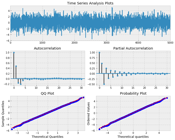 ARMA(2,2) processmdl = smt.ARMA(arma22, order=(2, 2)).fit( maxlag=max_lag, method=’mle’, trend=’nc’, burnin=burn)print(mdl.summary()) ARMA Model Results ====================================================================Dep. Variable: y No. Observations: 5000Model: ARMA(2, 2) Log Likelihood -7054.211Method: mle S.D. of innovations 0.992Date: Mon, 27 Feb 2017 AIC 14118.423Time: 21:27:58 BIC 14151.009Sample: 0 HQIC 14129.844 ==================================================================== coef std err z P>|z| [0.025 0.975]——————————————————————–ar.L1.y 0.5476 0.058 9.447 0.000 0.434 0.661ar.L2.y -0.2566 0.015 -17.288 0.000 -0.286 -0.228ma.L1.y 0.4548 0.060 7.622 0.000 0.338 0.572ma.L2.y -0.3432 0.055 -6.284 0.000 -0.450 -0.236 Roots ==================================================================== Real Imaginary Modulus Frequency——————————————————————–AR.1 1.0668 -1.6609j 1.9740 -0.1591AR.2 1.0668 +1.6609j 1.9740 0.1591MA.1 -1.1685 +0.0000j 1.1685 0.5000MA.2 2.4939 +0.0000j 2.4939 0.0000——————————————————————–
If you run the above code a few times, you may notice that the confidence intervals for some coefficients may not actually contain the original parameter value. This outlines the danger of attempting to fit models to data, even when we know the true parameter values!
However, for trading purposes we just need to have a predictive power that exceeds chance and produces enough profit above transaction costs, in order to be profitable in the long run.
So how do we decide the values of p and q ?
We exapnd on the method described in previous sheet. To fit data to an ARMA model, we use the Akaike Information Criterion (AIC)across a subset of values for p,q to find the model with minimum AIC and then apply the Ljung-Box test to determine if a good fit has been achieved, for particular values of p,q. If the p-value of the test is greater the required significance, we can conclude that the residuals are independent and white noise.
# Simulate an ARMA(3, 2) model # alphas=[0.5,-0.4,0.25] # betas=[0.5,-0.3]max_lag = 30n = int(5000)burn = 2000alphas = np.array([0.5, -0.4, 0.25])betas = np.array([0.5, -0.3])ar = np.r_[1, -alphas]ma = np.r_[1, betas]arma32 = smt.arma_generate_sample(ar=ar, ma=ma, nsample=n, burnin=burn)_ = tsplot(arma32, lags=max_lag)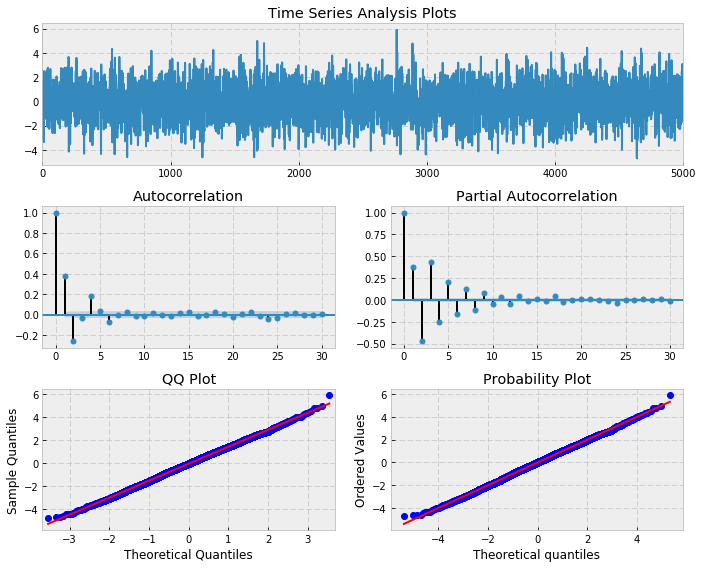 ARMA(3,2) model# pick best order by aic # smallest aic value winsbest_aic = np.inf best_order = Nonebest_mdl = Nonerng = range(5)for i in rng: for j in rng: try: tmp_mdl = smt.ARMA(arma32, order=(i, j)).fit(method=’mle’, trend=’nc’) tmp_aic = tmp_mdl.aic if tmp_aic < best_aic: best_aic = tmp_aic best_order = (i, j) best_mdl = tmp_mdl except: continueprint(‘aic: %6.2f | order: %s’%(best_aic, best_order))
aic: 14110.88 | order: (3, 2)
sms.diagnostic.acorr_ljungbox(best_mdl.resid, lags=[20], boxpierce=False)
(array([ 11.602271]), array([ 0.92908567]))
Notice that the p-value is greater than 0.05, which states that the residuals are independent at the 95% level and thus an ARMA(3,2) model provides a good model fit (ofcourse, we knew that).
Let?s also check if the model residuals are indeed white noise
_ = tsplot(best_mdl.resid, lags=max_lag)from statsmodels.stats.stattools import jarque_berascore, pvalue, _, _ = jarque_bera(mdl.resid)if pvalue < 0.10: print ‘The residuals may not be normally distributed.’else: print ‘The residuals seem normally distributed.’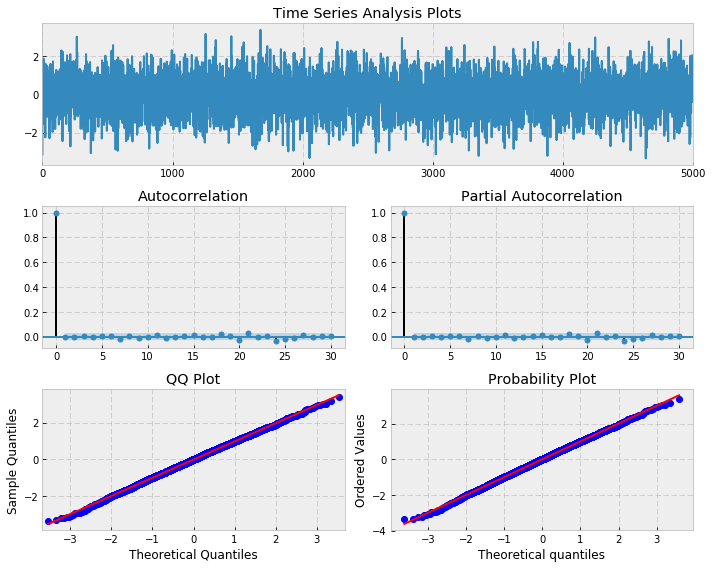 Residuals after finding best fit for ARMA(3,2)The residuals seem normally distributed.
Finally, let?s fit an ARMA model to SPX returns.
import auquanToolbox.dataloader as dl# download dataend = ‘2015-01-01’start = ‘2007-01-01’symbols = [‘SPX’,’DOW’,’AAPL’,’MSFT’]data = dl.load_data_nologs(‘nasdaq’, symbols , start, end)[‘ADJ CLOSE’]# log returnslrets = np.log(data/data.shift(1)).dropna()# Fit ARMA model to SPY returnsbest_aic = np.inf best_order = Nonebest_mdl = Nonerng = range(5) # [0,1,2,3,4,5]for i in rng: for j in rng: try: tmp_mdl = smt.ARMA(lrets.SPX, order=(i, j)).fit( method=’mle’, trend=’nc’) tmp_aic = tmp_mdl.aic if tmp_aic < best_aic: best_aic = tmp_aic best_order = (i, j) best_mdl = tmp_mdl except: continueprint(‘aic: {:6.2f} | order: {}’.format(best_aic, best_order))_ = tsplot(best_mdl.resid, lags=max_lag)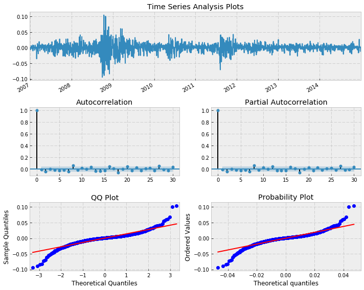 Residuals after fitting ARMA(3,2) to SPX returns from 2007?2015aic: -11515.95 | order: (3, 2)
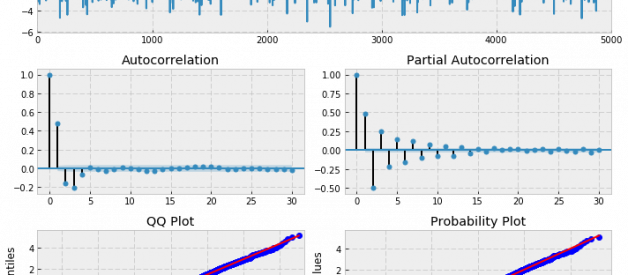
The best fitting model has ARMA(3,2). Notice that there are some significant peaks, especially at higher lags. This is indicative of a poor fit. Let?s perform a Ljung-Box test to see if we have statistical evidence for this:
sms.diagnostic.acorr_ljungbox(best_mdl.resid, lags=[20], boxpierce=False)
(array([ 39.20681465]), array([ 0.00628341]))
As we suspected, the p-value is less that 0.05 and as such we cannot say that the residuals are a realisation of discrete white noise. Hence there is additional autocorrelation in the residuals that is not explained by the fitted ARMA(3,2) model. This is obvious from the plot of residuals as well, we can see areas of obvious conditional volatility (heteroskedasticity) that the model has not captured.
In the next post, we will take this concept of merging AR and MA models even further and discuss ARIMA models.
We will also finally talk about how everything we?ve learned so far can be used for forecasting future values of any time series. Stay tuned!

