UPDATE: Algorithm is now licensed under WTFPLv2. Source codes available at https://github.com/schizofreny/middle-out.
Middle-out compression is no longer a fictional invention from HBO?s show Silicon Valley. Inspired by both the TV show and new vector instruction sets, we came up with a new lossless compression algorithm for time-series data. Compression is always about a compromise between speed and ratio and It is never easy to balance these trade-offs, but the whole middle-out concept allows us to push Weissman score even further.
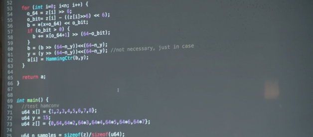
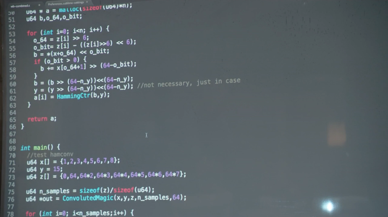 Source code of Pied Paper?s compression algorithm
What Is So Special about Middle-Out Compression?
It simply breaks data dependency. If we need a previous value to compute a current one, we need all antecedent values. But if we start processing from multiple positions of the chunk we depend only on antecedent values within this fragment. This allows us, for instance, to effectively use SIMD instructions.
How Does it Work?
In principle, the algorithm computes the XOR of a new value and the previous one. This way we get a sort of diff between values and we can store this diff alone. In time-series datasets this diff typically has a number of either leading and/or trailing zeroes. Hence the information we need to store is usually significantly smaller, but we also need to store leading zeros count and length of non-zero XOR fragment.
These concepts are generally used in current compressions algorithms, e.g. Facebook?s Gorilla [1]. For the sake of compression efficiency, Gorilla operates on bits level, but these operations are quite expansive. We have designed our compression to be as fast as possible so we moved from bit to byte granularity. As a consequence, one would expect worse compression ratio, but that is not always the case.
With regard to middle-out, compression operates on blocks of data, but this is not a problem as time-series databases uses blocks anyway.
What About Compression Ratio?
Let?s examine compression ratio in two different scenarios. The first scenario ? we take a series of doubles (i.e. 0.1, 0.2, 0.3, ?) and measure compression ratio depending on the portion of repeating points. For comparison we use Facebook?s Gorilla compression. By default Gorilla compresses both the values and timestamps of time-series data. For our test purposes, compression of timestamps is disabled.
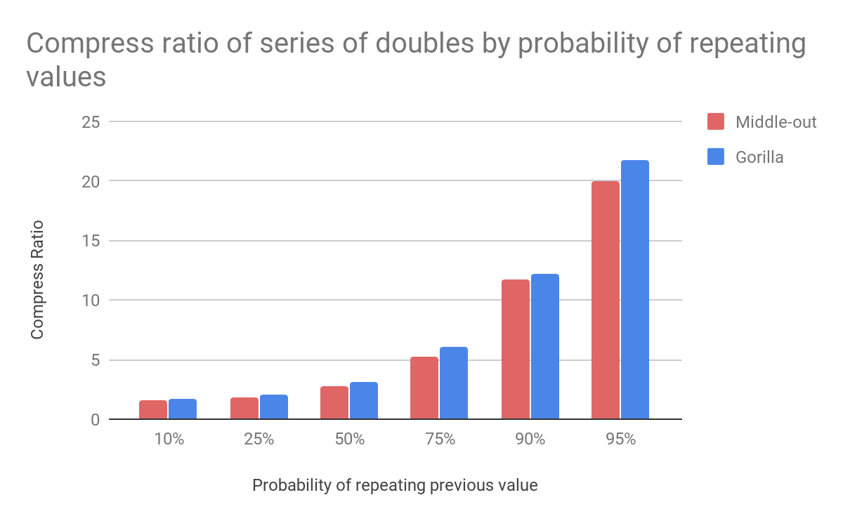
It isn?t surprising to find that Gorilla has slightly better compression ratio for these types of data. We can see the same trend with long-integer sequences.
Second scenario ? datasets. Datasets A and B share the same minute stock data. In the case of dataset A, price points are compressed as floating point numbers. In dataset B these numbers are first multiplied to shift the decimal point and hence we can represent these numbers as long without losing precision.
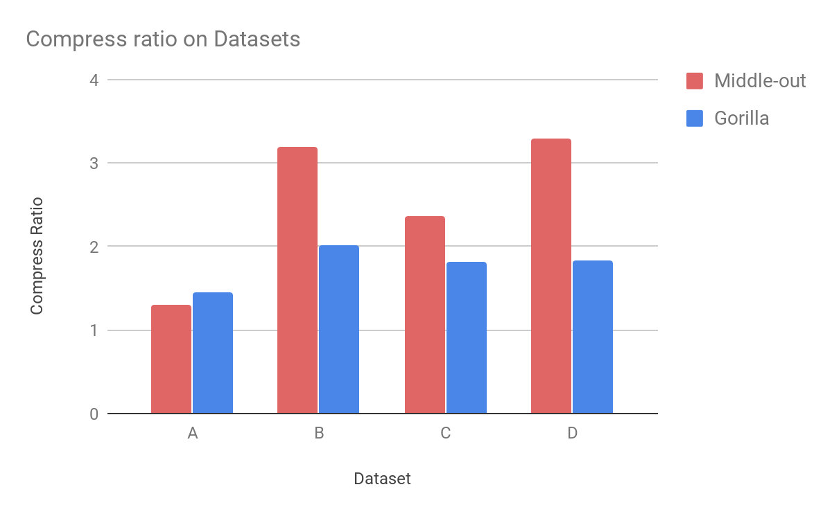
Datasets C and D are generated using a benchmarking tool from InfluxData [2]: representing disk writes and redis memory usage. In the case of dataset A, Gorilla compresses data slightly better than our algorithm ? with a ratio of 1.45 vs 1.3. Other datasets using integers are better compressed with our new algorithm. The biggest difference can be seen in dataset D where the Middle-out compression ratio is 3.3, whereas Gorilla can compress these data only with a ratio of 1.84. Compression ratio substantially depends on the input of data and there are obviously datasets where one algorithm compresses better than another. But if performance is your concern ? keep reading.
Compression Performance
Currently we have two compatible implementations of the algorithm. One utilizes a new AVX-512 instruction set available on Skylake-X CPUs. The second implementation targets computers without the support of this instruction set.
Throughput is measured on a single core of Skylake-X running at 2.0 GHz.
The following charts show the compression and decompression speed of both implementations compared to Facebook?s Gorilla.
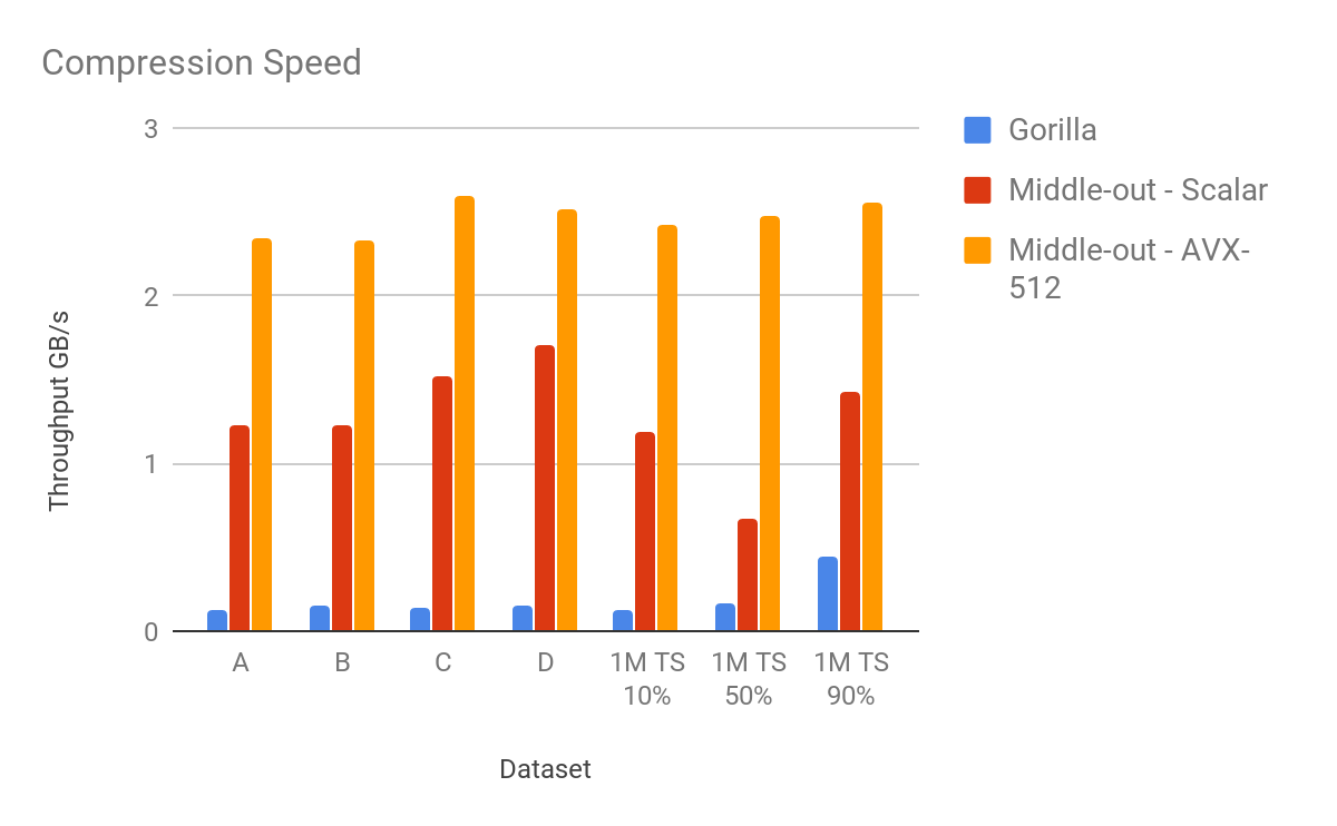
This graph shows compression throughput as measured on the four datasets discussed above, plus the throughput of a series with the respective percentage of repeating values.
The throughput of Gorilla compression varies from 120?440 MB/s with an average speed of 185 MB/s. The lowest throughput of our scalar implementation compresses around 670 MB/s for 50% of repeating values. This is due to a high branch misprediction ratio. The average compression speed is 1.27 GB/s. An algorithm using vector instructions does not suffer from branch misprediction and compresses data from 2.33 GB/s to 2.59 GB/s, with an average speed of 2.48 GB/s. Not bad for a single core of 2 GHz chip.
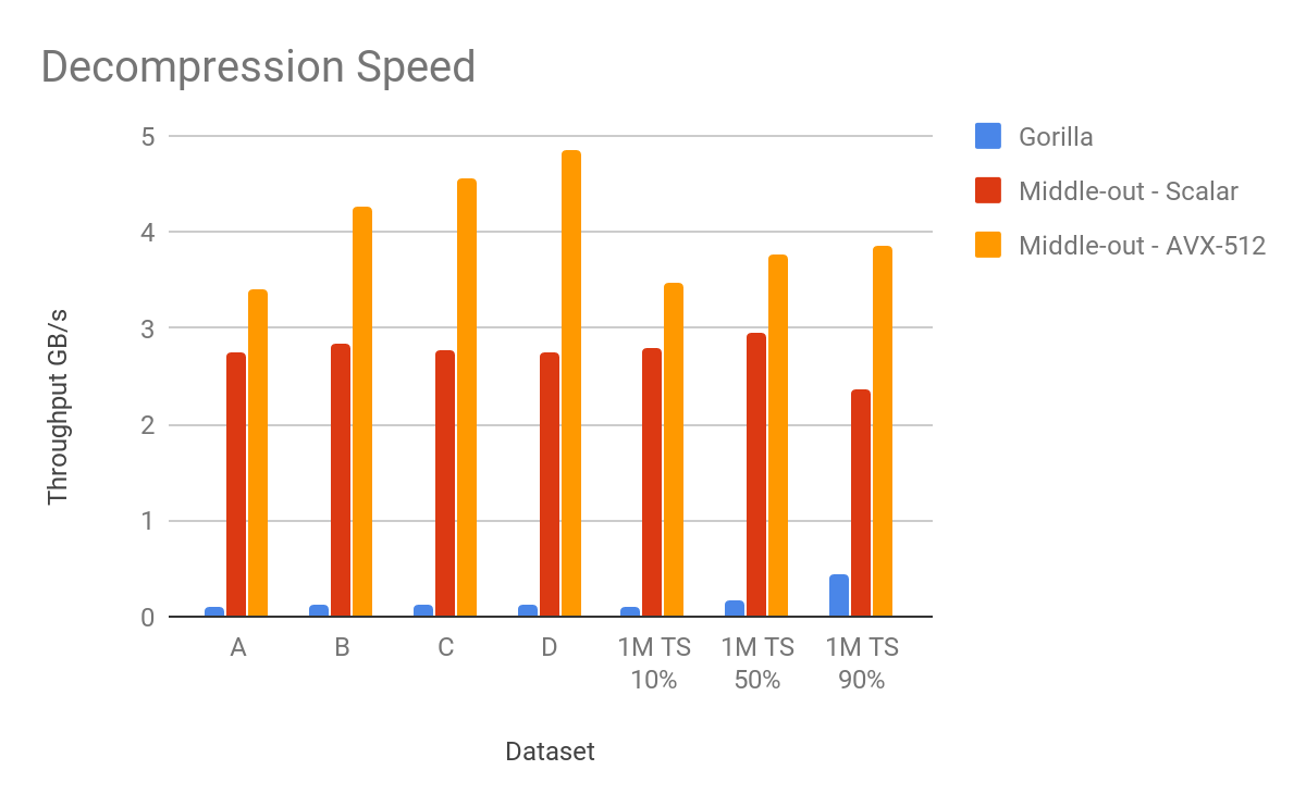
Gorilla can decompress these data at speeds ranging from 100 MB/s to 430 MB/s . But as you can see, our decompression of the same data is even faster than a compression. Non-vectorized decompression operates at a minimal speed of 2.36 GB/s and 2.7 GB/s on average. Vectorized codes decompress data from 3.4 GB/s, hitting 4.86 GB/s for dataset D. On average it is able to decompress the data at 4.0 GB/s.
The average overall speedup for compression is 6.8x (scalar implementation) and 13.4x (vectorized implementation). The average speedup for decompression is 16.1x and 22.5x respectively.
About us
We at Schizofreny are devoted to performance and we believe that limits can always be pushed further. We love challenges and we are here to help with your HPC problems.
Part II
[1] www.vldb.org/pvldb/vol8/p1816-teller.pdf
[2] https://github.com/influxdata/influxdb-comparisons/
