Optimization, one of the elementary problems of mathematical physics, economics, engineering, and many other areas of applied math, is the problem of finding the maximum or minimum value of a function, called the objective function, as well as the values of the input variables where that optimum value occurs. In elementary single-variable calculus, this is a very simple problem that amounts to finding the values of x for which df/dx is zero.
Multivariable optimization problems are more complicated because we can impose constraints. We consider constraints that can be expressed in the form g(x,y,z)=c for some function g and constant c. These are called equality constraints, and the set of points satisfying these constraints is called the feasible set, which we denote by S. For example, if we are asked to find the maximum value of f(x,y) on the unit circle, then g(x,y)=x+y since the unit circle is defined by x+y=1.
The standard technique for solving this kind of problem is the method of Lagrange multipliers. In this article, I will derive the method and give a few demonstrations of its use.
Motivation and derivation
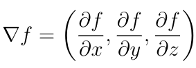
A function f has a local extremum (maximum or minimum) at a point P when the partial derivative of f is zero for each of the independent variables and when the point is not a saddle point (a situation which we won?t need to spend any time dealing with here). We can write this in compact form as ?f=0, where ? denotes the gradient operator:
In constrained optimization, however, just because f has a local maximum or minimum at a point on the feasible set, it does not follow that f takes its optimal value on the feasible set at that point.
As an example, let?s consider the following optimization problem:
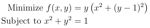
By writing out the gradient, we can see that f has a local minimum when x=0 and y=1:
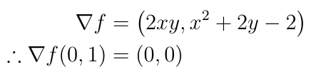
Furthermore, f(0,1)=0, but f(0,-1)=-4 so although (0,1) is a local minimum of f(x,y), it is not the minimum of f(x,y) on the unit circle.
As another example, let?s maximize f(x,y)=y on the unit circle. The gradient of f(x,y)=y is a constant vector so f(x,y) has no local maxima or minima, but on the unit circle f does have a maximum value of 1, occurring at (0,1).
The reason for this failure is that the gradient measures the rate of change of f(x,y,z) with respect to position in three-dimensional space, but we want to measure the rate of change of f(x,y,z) with respect to position in the feasible set. For a three-dimensional problem, S will be either a curve or a surface, and in general for problems with n variables, S will be a hypersurface of dimension strictly less than n.
The most natural approach is to consider curves in S. Let P be a point in S for which f(P) takes a locally optimal value in S but ?f(P) is not necessarily zero, and let r(t) be the parameterization of any curve in S that passes through P, that is:
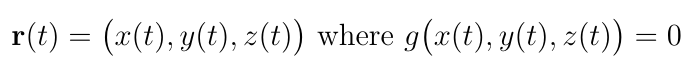
If S is a curve, then r(t) is just a parameterization of S. Furthermore, let r(T)=P, r?(T)?0, and let h(t) = f(r(t)) so that h?(T)=0. Let?s expand h?(t) using the chain rule:
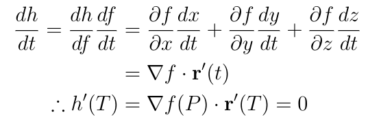 Note that in the first line, I used the fact that dh/df=1.
Since r(t) is always in S, the velocity vector r?(t) must always be tangent to the surface or curve of S since if r?(t) had a component perpendicular to the surface, that is, directed out from the surface, then there would be points where r(t) leaves S. Since this is true of any curve r(t) that passes through P, it follows that ?f(P) is perpendicular to any tangent vector to the surface at P. So if P is a point where f takes a maximum or minimum value with respect to position in S, then ?f(P) is perpendicular to S.
The converse is also true: Since r?(T) is never zero and always parallel to S, then if ?f(P) is perpendicular to S, then h?(T)=?f(P)?r?(T)=0.
But how do we actually find points where ?f is perpendicular to S? Here is the answer: The set S is the set of all points where g(x,y,z)=c, that is, S is a level set of g. This means that ?g is perpendicular to S for all points in S, so ?f and ?g are parallel at points in S where f takes optimal values. This means that f takes its optimal values in S precisely when ?f=??g for some constant ?. The constant ? is called the Lagrange undetermined multiplier, and this is where the method gets its name. The problem of optimizing f can now be solved by finding four unknowns x, y, z, and ? that solve these four equations:
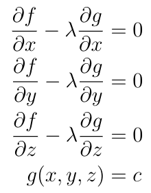
Put another way, our goal now is to optimize the function f-?g with respect to x, y, and z without constraints by finding where ?(f-?g)=0.
What if there is more than one constraint? Suppose now that we have to optimize f(x,y,x) subject to g(x,y,z)=c and h(x,y,z)=d. Here is what we do. To optimize f subject to g(x,y,z)=c, we optimize f-?g without constraint, so the first constraint is taken care of by replacing f with f-?g, and it remains to optimize f-?g subject to the constraint h(x,y,z)=d. This is a problem with just one constraint, so we simply add another Lagrange multiplier ?, and the problem now is to optimize f-?g-?h without constraint.
Let?s now look at some examples.
The maximum area of a rectangle
For a given perimeter, what is the greatest possible area of a rectangle with that perimeter? We can formulate this as a Lagrange multiplier problem. If the width and height are x and y, then we wish to maximize f(x,y)=xy for g(x,y)=2x+2y=c. The resulting system of equations is:
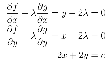
The first two equations tell us right away that x=y, so the maximum area occurs when the rectangle is a square. By plugging this into the the third equation, we see that x=y=c/4, so the maximum area of a rectangle with perimeter c is c/16.
A (modified) Putnam problem
The Putnam mathematical competition is an exam-format competition offered every December to undergraduate students. Students have six hours to solve 12 extremely challenging problems. The exam is so difficult that, out of a possible score of 120, the average score in most years is 0 or 1. Today we?ll be looking at a modified version (for simplicity and to avoid copyright issues) of problem A3 from the 2018 exam:
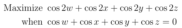
There are two problems. The first is that the objective function has a very undesirable feature: it?s a sum of cosines, and sums of trig functions can be tough to deal with. The second is that there is no way to make the constraint function appear neatly and explicitly in the objective function, even though at first glance it might seem like this should be possible. Putnam problems often involve ?traps? like this, where you can be lured into wasting time on an approach that will not lead to a solution if you don?t stop to think about what you?re doing. It?s a trap that would be especially hazardous to a contestant with experience in high school math competitions, where trig identities tend to be a strong emphasis.
But when we see a problem that says ?maximize f subject to g=0?, we should immediately think about Lagrange multipliers. Let?s set up our system of equations:
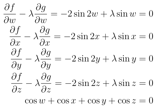
Now we can use our trig identities to make the constraint appear explicitly. Rewrite the system of equations using the double-angle formula:
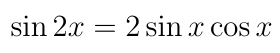
The result is:
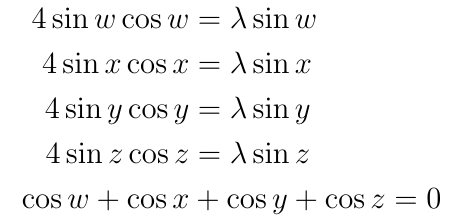
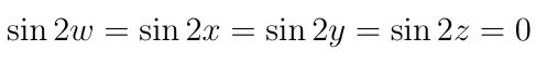
Now cancel the sine function on each side, and add the equations:
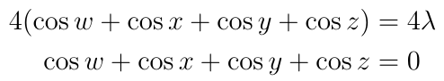
And this means that ?=0, so according to the Lagrange multiplier equations this means that:
Therefore w, x, y, and z are all integer multiplies of ?/2. For even integer multiplies of ?/2, say m=2k for some integer k:
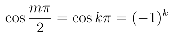
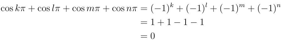
But if m is an odd integer, then cos(m?/2)=0. This means that we have three options for how we can satisfy the constraint equation. First, we can set w, x, y, and z all to odd integer multiplies of ?/2, say k, l, m, and n, then:
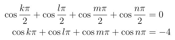
The first line is showing that the constraint equation is satisfied, and the second line is the result of plugging those values in to the objective function, which gives us -4.
The second option is that we can set two of the variables to odd integer multiples of ?/2, say k and l, and the other two to even integers, say 2m and 2n where m is even and n is odd. The result of plugging this into the constraint equation is:
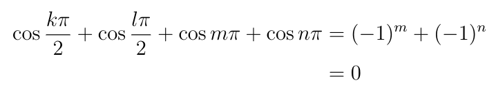
So the constraint equation is satisfied. Here is the result of plugging these into the objective function:

The final option is that we can set all of the variables to even integer multiplies of ?/2, say 2k, 2l, 2m, and 2n, where k and l are even and m and n are odd. The result of plugging this into the constraint equation is:
So the constraint is satisfied. Now we plug these into the objective function to get:

So the answer is 4, which coincidentally turns out to be the global maximum value of the objective function.
Check out this other article I wrote for a discussion of another Putnam problem.
Thomson?s Theorem
Now instead of optimizing a function, let?s use the method of Lagrange multipliers to optimize a functional: an object that takes a function and returns a number. Definite integrals are a key example. This final demonstration will show how the method of Lagrange multipliers can be used to find the function that minimizes the value of a definite integral.
As a demonstration, we consider a fundamental fact from electrostatics, the study of systems subject to electric forces in mechanical equilibrium so that none of the charges are in motion. We will show that when a conductor, a body in which electric charge can move freely, is in equilibrium with any system of electric forces, then there is no electric field inside the body of the conductor. This is Thomson?s Theorem. This theorem is usually stated in terms of the fundamental physical fact that the energy of a system in stable mechanical equilibrium is minimal:
Thomson?s Theorem: The electrostatic energy of a conducting body of fixed size and shape is minimized when the charges are distributed in such a way as to make the potential ? constant in the body so that E=-??=0.
Let ?(r) be the charge distribution function and ???? the potential due to any sources external to the conducting body. The total electrostatic energy can be expressed as a functional U of ?(r):
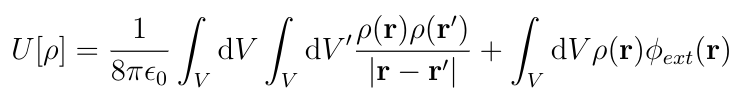
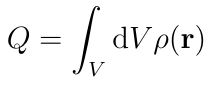
These are volume integrals over the body of the conductor. The first integral is a double integral carried out first over the primed coordinates and then over the unprimed coordinates. We want to minimize U as a functional of ?(r) given that the total charge is independent of the charge distribution:
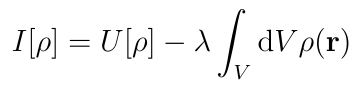
Fortunately, the method of Lagrange multipliers works for functionals with constraints. Introduce a Lagrange undetermined multiplier, and then rather than constrained optimization on U[?], perform unconstrained optimization on the following functional:
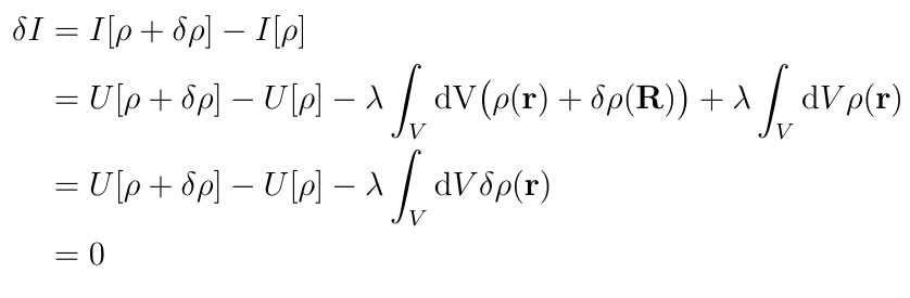
By analogy with derivatives of functions, the goal here is to find the charge distribution ? such that when ? is varied by a small variation ??, the change in I, ?I, is zero:
This isn?t quite a derivative because ?? is a function rather than a number so it doesn?t really make sense to speak of the limit as ?? goes to zero, but the basic intuition is the same.
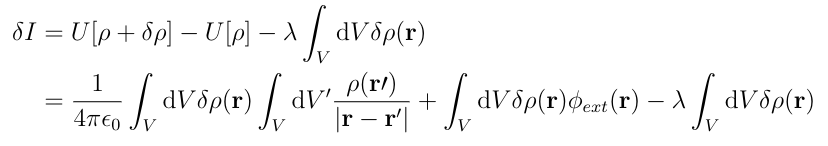
Let?s start by expanding U[?+??]:
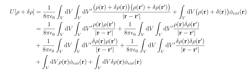
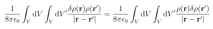
This may look bad, but we can simplify this greatly. First, since ?? is very small, (??) is so small that we can ignore it, so assume that ??(r)??(r?)=0. Next, by changing the order of integration we see that:
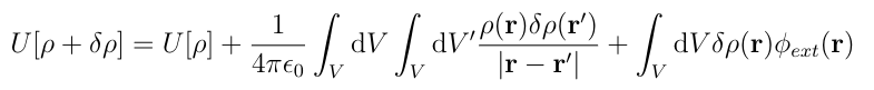
We can also see that U[?] appears in the expansion. This gives us enough to simplify U[?+??]:
Now we can expand ?I:
Now we can factor out the integral over ??(r):
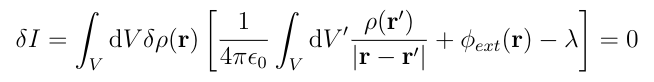
For this to be true for any choice of the variation ??(r), the bracketed term must be zero, so:
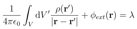
But this integral is just the potential at r due to the charges inside the conductor so the left hand side of this equation gives the total potential at every point r inside the conductor, so ?(r) is the distribution that makes the total potential inside of the conductor constant. This completes the proof.
This would also be valid if the electrostatic energy of the conductor is maximized, in which case the conductor is in unstable equilibrium. In practice one never actually encounters conductors in unstable equilibrium because the random thermal motion of the electrons in the conductor will rapidly, on the order of 10?? seconds for metal conductors, drive the system out of unstable equilibrium and into stable equilibrium.
Conclusion, copyright stuff, etc
This has been my latest article on mathematical physics. If you enjoyed this then you may also enjoy my articles on Laplace?s equation and the heat equation, as well as my article about Feynman integration which I also linked in the second demonstration.
Any images in this article that are not cited are my own original work. The second example is based on problem A3 of the 2018 Putnam Exam, and the proof in the third example is based on the discussion on page 128 of Modern Electrodynamics by Zangwill (2013). These examples are used here in accordance with fair use guidelines.
EDIT: About an hour after posting this article I noticed significant issues with the second example so I decided to rewrite it with a slightly different example.

