The History of Euler’s Number (e)

From Napier Table?s To Bernoulli?s Compounding Interest

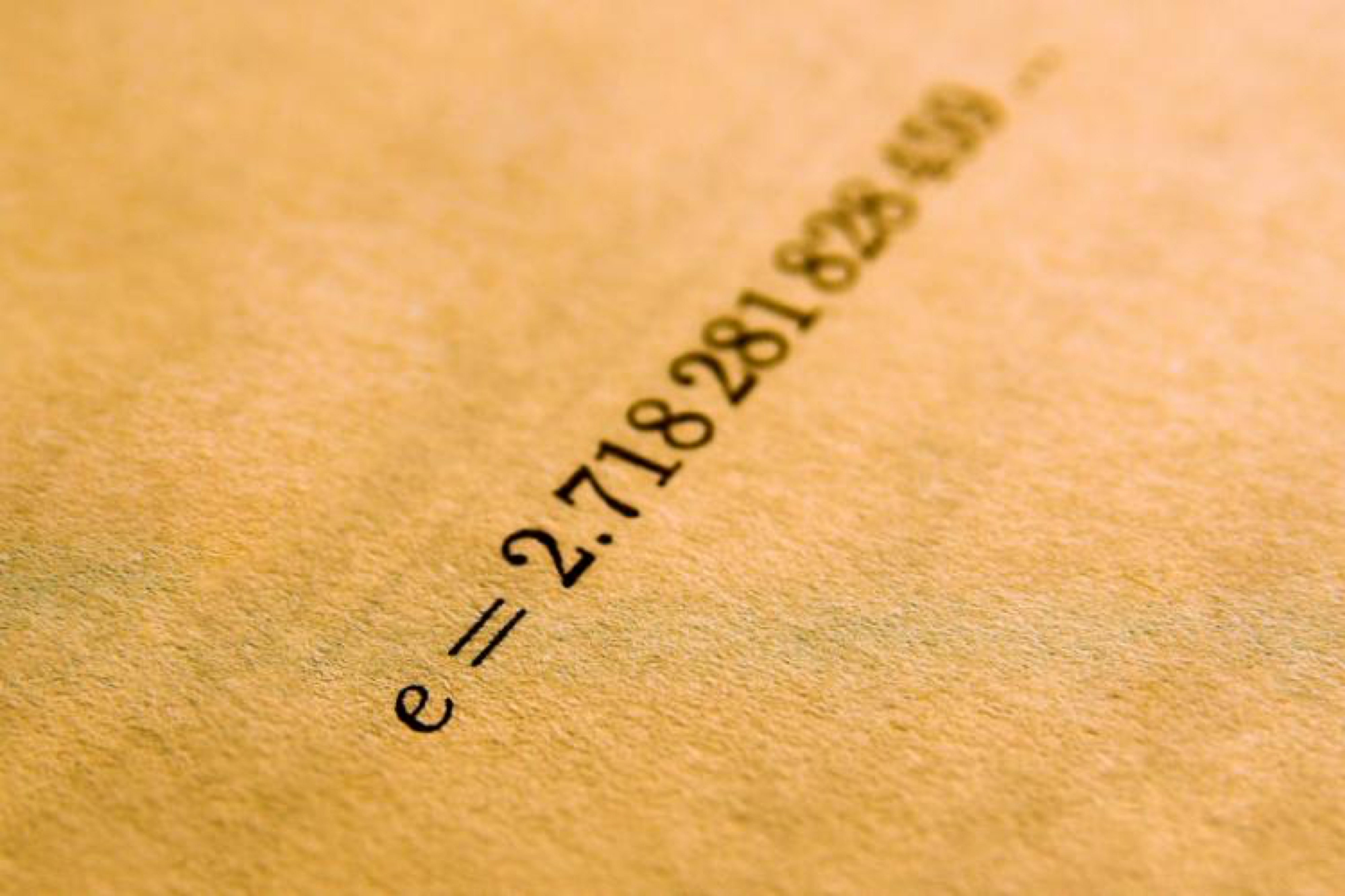
In math there are a few, select, magical constants that transverse all branches. These constants, steadily discovered throughout our collective history, provide the numerical infrastructure to our everyday lives; like chemical elements in the periodic table, special constants in math are foundational. To name a few, we have zero (0), circular-darling pi (~3.142), square-root of negative one (i) & of course, the exponential king, Euler?s constant ?e? (~2.718).

The focus of this piece, as accurately articulated by the title, is a deep dive into ?Euler?s number,? also known as ?Napier?s number? or more commonly, simply e. For the uninitiated, the number e is at the very crux of exponential relationships, specifically pertinent to anything with constant growth.

Just like every number can be considered a scaled version of 1 (the base unit) & every circle can be considered a scaled version of the unit circle (radius 1), every rate of growth can be considered a scaled version of e (unit growth, perfectly compounded). E is the base rate of growth shared by all continually growing processes; it shows up whenever systems grow exponentially & continuously: population, radioactive decay, interest calculations, etc? E represents the idea that all continually growing systems are scaled versions of a common rate.

Below, we?re going to visit the three individuals that contributed to its discovery: John Napier, Jacob Bernoulli & Leonard Euler.

Napier?s Logarithm

The first step to the discovery of e begins with one Scottish-polymath: John Napier. Far more comfortable inventing than theorizing, Napier?s contribution stems not from hardcore pure mathematics, but more so from a practical need: a computational shortcut when multiplying very large figures.

A common issue of his time, astronomers repeatedly observed potential new discoveries, yet they were plagued with interminably-large calculations which led to inaccuracy or abandonment of progress altogether. Like multiplication is a shortcut for addition & exponents are a shortcut for multiplication, Napier sought the next computational shortcut: a shortcut for exponents.

The basic idea of what logarithms were to achieve is straightforward: to replace the wearisome task of multiplying two numbers by the simpler task of adding together two other numbers. To each number, there was to be associated another, which Napier called at first an ?artificial number? & later a ?logarithm? (a term which he coined from Greek words), with the property that from the sum of two such logarithms the result of multiplying the two original numbers could be recovered.

Napier?s original discussion of logarithms appears in his Mirifici Logarithmorum Canonis Descriptio (published in 1614). Unlike the logarithms used today, Napier?s original logarithms are to base 1/e & involve a constant (10?). Napier defined his logarithms as a ratio of two distances in a geometric form, as opposed to the current definition of logarithms as exponents. While not the logarithm we use today, we?ll cover how Napier derived it below.

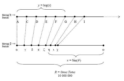
Napier grounded his conception of the logarithm in a kinematic framework. He imagined two particles traveling along two parallel lines; the first line was of infinite length & the second of a fixed length. Napier imagined the two particles to start from the same (horizontal) position at the same time with the same velocity. The first particle he set in uniform motion on the line of infinite length so that it covered equal distances in equal times. The second particle he set in motion on the finite line segment so that its velocity was proportional to the distance remaining from the particle to the fixed terminal point of the line segment.

Napier?s Parallel Lines w/ Moving Particles ? Landmarks of Science Series

More specifically, at any moment the distance not yet covered on the second (finite) line was the sine & the traversed distance on the first (infinite) line was the logarithm of the sine. This had the result that as the sines decreased, Napier?s logarithms increased. Furthermore, the sines decreased in geometric proportion, while the logarithms increased in arithmetic proportion. :

??=log???(??) where ?? = Sin?1

?? = log???(??) where ?? = Sin?2

More generally: ?=Sin(?) & ?=log???(?)

Continued Two-Particle Early Log

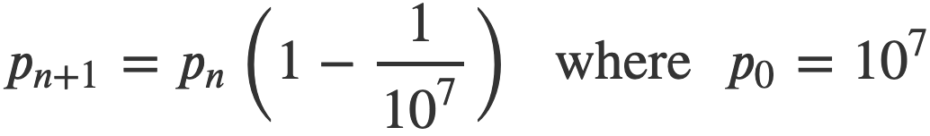
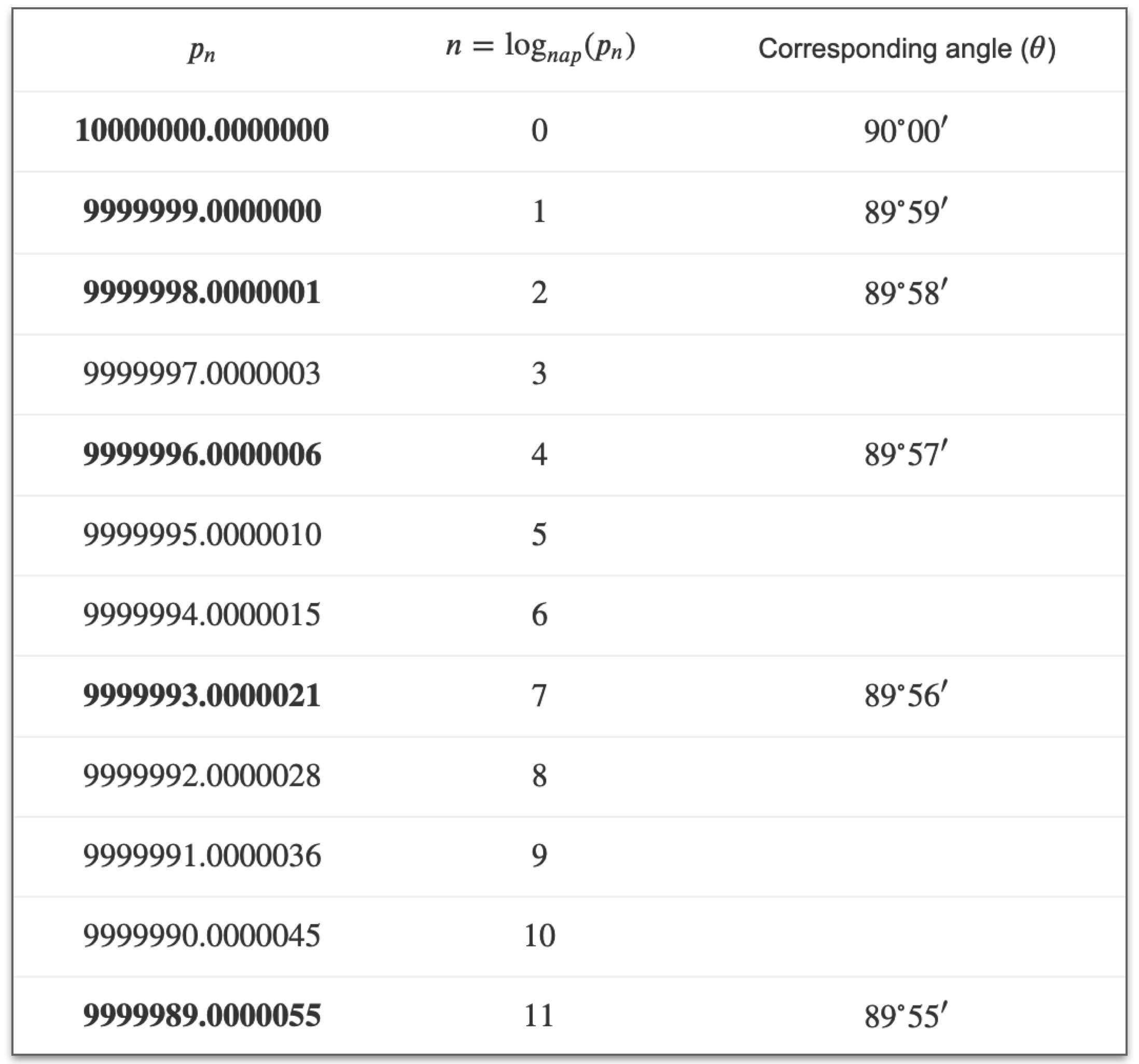
Napier generated numerical entries for a table embodying this relationship. He arranged his table by taking increments of arc ? minute by minute, then listing the sine of each minute of arc, & then its corresponding logarithm. For example, he would have computed values that appear in the first column of Table 1 via the relation:

Napier?s logarithms

The values in the first column correspond to the Sines of the minutes of arcs extracted in the third column, along with their accompanying logarithms placed in the middle second column. Circling back to Napier?s original work, the same table values above can be seen in the first six rows of the table below.

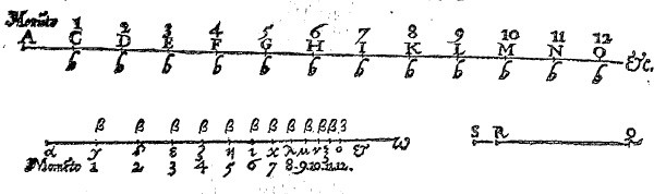
To complete his now-famous logarithm tables, Napier himself computed almost ten million entries from which he selected the appropriate values. Historical evidence supports that Napier dedicated himself at least twenty years to cumulatively creating the following tables:

Landmarks of Science Series, NewsBank-Readex

Again, it?s worth repeating that Napier?s original presentation of logarithms differed markedly from that generally adopted later. Mainly, most practitioners who had laborious computations generally did them in the context of trigonometry. Therefore, as well as developing the logarithmic relation, Napier set it in a trigonometric context so it would be even more relevant ? it?s connection to exponential growth, wouldn?t happen for a couple of decades.

Still, the fact remains that few mathematical inventions burst on the world so unexpectedly as Napier?s logarithms. Although various disparate strands ? the idea of doing multiplication via addition, the idea of comparing arithmetic & geometric progressions, the use of the concept of motion ? had all been floated at some stage, the enthusiasm with which Napier?s work was received makes it clear both that this was perceived as a novel invention & that it fulfilled a pressing need. Again though the possibility of defining logarithms as exponents, wouldn?t be recognized until Bernoulli & Euler came along.

Bernoulli?s Question

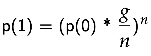
Appropriately enough, Jacob Bernoulli?s contribution to the discovery of e kicked off with a financial curiosity. At first a thought experiment, he pondered how compounding growth at alternating time periods, but with the same rate, changes the principal output. This next series of examples all use the standard annual growth formula:

Bernoulli?s logic is elementary to follow ? imagine an example bank account A, that starts with $1.00 & pays 100% interest per year (yes this rate is unrealistic but it provides us with simple math). The principle value at the end of the year is simple: $2.00 ((1+(1/1)). But now, instead of compounding once for the full 100%, let?s compound twice (semi-annually) with 50% growth each period ? the final figure is now a higher $2.25 ((1+(.5))). How about if we compound three times with 33.33% growth? The yielding principle is an even higher $2.37 (((1+(.33))). And finally, what if we calculated the final principle with quarterly compounding? We?d receive $2.44 (((1+(.25))? )at year?s end.

As Bernoulli (& hopefully you) noticed, increasing the frequency of compounding periods, yet leaving the rate of growth as equal, increases our output principle; however, the output principle is increasing at a decreasing rate. For example, compounding semi-annually led to a 12.5% increase (from $2.00), compounding every four-months led an 18.5% increase, & quarterly compounding led to a 22% increase. Each trial with an increase in compounding periods leads to an increase in the output principle, however, this increase is growing at a decreasing rate.

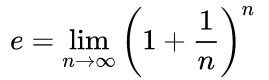
This hint at convergence on long-enough timeline clues us into the fact that we?re dealing with an infinite series, so we turn to our handy-calculus tool of finding limits. As Bernoulli himself pondered, what happens to our principle when we compound at ever-faster frequencies ? say if we compounded weekly ($2.69) or even daily ($2.72)? It?s obvious that compounding more frequently results in more money in the bank, so it is natural to ask what happens when interest is compounding at every instant in time (that is, continuously)?

Using n as the number of compounding intervals, with interest of 100% in each interval, Bernoulli set up a limit function that Euler would pick up a few ~40 years afterward:

Bernoulli is credited with writing e down for the first time, as he did indeed manually approach the value of e (2.718281) through the exercise above; it wasn?t until Euler, however, that the significance of e was truly unlocked & inserted into everyday math lingo.

Euler?s Answer

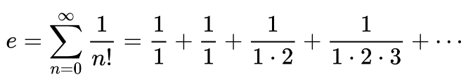
Shockingly, Leonard Euler had very little to do with the number e outside of attaching its memorable namesake. His one, true, technical contribution came from proving that e is irrational by re-writing it as a convergent infinite series of factorials:

His second contribution, the core reason the constant bears his initial, is simply because he famously used the constant in a letter to a colleague & historically declared it as e. It?s now a happy coincidence that ?e? is the first letter in exponential, however, the jury is still out on whether he purposefully named it after himself. The truth may be even more prosaic: Euler was using the letter a in some of his other mathematical work, and e was the next vowel.

Whatever the reason, the notation e made its first appearance in a letter Euler wrote to Goldbach in 1731. He made various discoveries regarding e in the following years, but it was not until 1748 when Euler published Introductio in Analysin infinitorum that he gave a full treatment of the ideas surrounding e.

Courtesy of A Personal Hero ? Numberphile/Youtube

In Closing

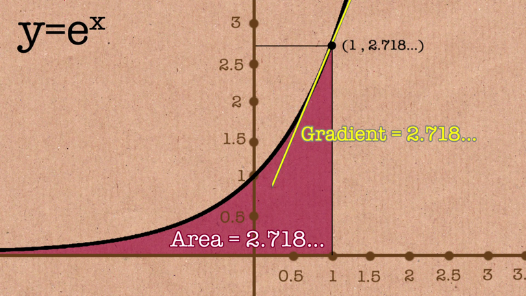
Like ?, e is derivable, yet it maintains its mystical appeal. Take a moment to really grasp the above ? if we graph the equation y=e^x we find that:

1. The slope of that curve at any given point is also e^x
2. The area under the curve from negative infinity up to x is also e^x

E & the function of e^x is the only constant in all of mathematics in which the two points above hold true. It?s significant, because, once again, it showcases how intimately e is intertwined with the relationship of consistent growth. Like other beautiful, perfect constants that repeatedly show up in this shared reality of ours, it?s incredibly fun & rewarding to continue digging under our fabric for further understanding. And who knows how many other special numbers are out there? Our universe is infinite, so it?s highly unlikely that we?ve discovered all structurally-critical constant; perhaps, a century from now, pi & e will only be one of many mystery numbers.