

Portfolio optimization is the process of selecting the best portfolio (asset distribution),out of the set of all portfolios being considered, according to some objective. The objective typically maximizes factors such as expected return, and minimizes costs like financial risk.-Wikipedia
In this article I will show you how to create a program to optimize a stock portfolio using the efficient frontier & Python ! In modern portfolio theory, the efficient frontier is an investment portfolio which occupies the ?efficient? parts of the risk-return spectrum. Formally, it is the set of portfolios which satisfy the condition that no other portfolio exists with a higher expected return but with the same standard deviation of return.
The Sharpe Ratio goes further: it actually helps you find the best possible proportion of these stocks to use, in a portfolio. – Moneychimp
The Sharpe ratio was developed by William F. Sharpe in 1966. The ratio describes how much excess return you receive for the extra volatility you endure for holding a riskier asset. It measures the performance of an investment compared to a risk-free asset (bonds, treasury bills, etc.), after adjusting for its risk. It is defined as the difference between the returns of the investment and the risk-free return, divided by the standard deviation of the investment.-Investopedia
So what is considered a good Sharpe ratio that indicates a high degree of expected return for a relatively low amount of risk?
Usually, any Sharpe ratio greater than 1.0 is considered acceptable to good by investors. A ratio higher than 2.0 is rated as very good. A ratio of 3.0 or higher is considered excellent. A ratio under 1.0 is considered sub-optimal.
If you prefer not to read this article and would like a video representation of it, you can check out the YouTube Video . It goes through everything in this article with a little more detail, and will help make it easy for you to start programming even if you don?t have the programming language Python installed on your computer. Or you can use both as supplementary materials for learning !
Programming:
The first thing that I like to do before writing a single line of code is to put in a description in comments of what the code does. This way I can look back on my code and know exactly what it does.
# Description: This program attempts to optimize a users portfolio using the Efficient Frontier & Python.
Import the libraries.
# Import the python librariesfrom pandas_datareader import data as webimport pandas as pdimport numpy as npfrom datetime import datetimeimport matplotlib.pyplot as pltplt.style.use(‘fivethirtyeight’)
Create The Fictional Portfolio
Get the stock symbols / tickers for the fictional portfolio. I am going to use the five most popular and best performing American technology companies known as FAANG, which is an acronym for Facebook, Amazon , Apple, Netflix , & Alphabet (formerly known as Google).
assets = [“FB”, “AMZN”, “AAPL”, “NFLX”, “GOOG”]
Next I will assign equivalent weights to each stock within the portfolio, meaning 20% of this portfolio will have shares in Facebook (FB), 20% in Amazon (AMZN), 20% in Apple (AAPL) , 20% in Netflix (NFLX), and 20% in Google (GOOG).
This means if I had a total of $100 USD in the portfolio, then I would have $20 USD in each stock.
# Assign weights to the stocks. Weights must = 1 so 0.2 for eachweights = np.array([0.2, 0.2, 0.2, 0.2, 0.2])weights
Now I will get the stocks starting date which will be January 1st 2013, and the ending date which will be the current date (today).
#Get the stock starting datestockStartDate = ‘2013-01-01’# Get the stocks ending date aka todays date and format it in the form YYYY-MM-DDtoday = datetime.today().strftime(‘%Y-%m-%d’)
Time to create the data frame that will hold the stocks Adjusted Close price.
#Create a dataframe to store the adjusted close price of the stocksdf = pd.DataFrame()#Store the adjusted close price of stock into the data frame for stock in assets: df[stock] = web.DataReader(stock,data_source=’yahoo’,start=stockStartDate , end=today)[‘Adj Close’]
Show the data frame and the adjusted close price of each stock.
df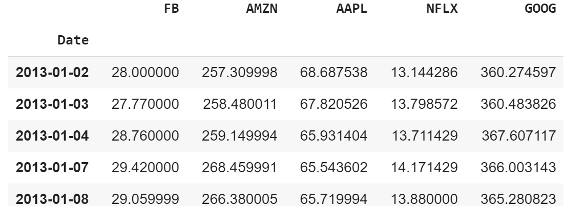
Visually show the stock prices.
# Create the title ‘Portfolio Adj Close Price Historytitle = ‘Portfolio Adj. Close Price History ‘#Get the stocksmy_stocks = df#Create and plot the graphplt.figure(figsize=(12.2,4.5)) #width = 12.2in, height = 4.5# Loop through each stock and plot the Adj Close for each dayfor c in my_stocks.columns.values: plt.plot( my_stocks[c], label=c)#plt.plot( X-Axis , Y-Axis, line_width, alpha_for_blending, label)plt.title(title)plt.xlabel(‘Date’,fontsize=18)plt.ylabel(‘Adj. Price USD ($)’,fontsize=18)plt.legend(my_stocks.columns.values, loc=’upper left’)plt.show()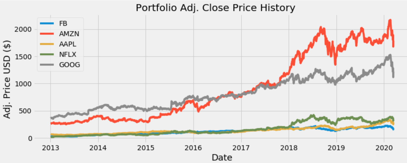
Financial Calculations
I?m done creating the fictional portfolio. Now I want to show the daily simple returns which is a calculation of the (new_price + -old_price)/ old_price or (new_price / old_price)-1.
#Show the daily simple returns, NOTE: Formula = new_price/old_price – 1returns = df.pct_change()returns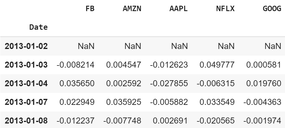
Create and show the annualized co-variance matrix. The co-variance matrix is a mathematical concept which is commonly used in statistics when comparing data samples from different populations and is used to determine how much two random variables vary or move together (so it?s the directional relationship between two asset prices ).
The diagonal of the matrix are the variances and the other entries are the co-variances. Variance is a measure of how much a set of observations differ from each other. If you take the square root of variance you get the volatility also known as the standard deviation.
To show the annualized co-variance matrix we must multiply the co-variance matrix by the number of trading days for the current year. In this case the number of trading days will be 252 for this year.
cov_matrix_annual = returns.cov() * 252cov_matrix_annual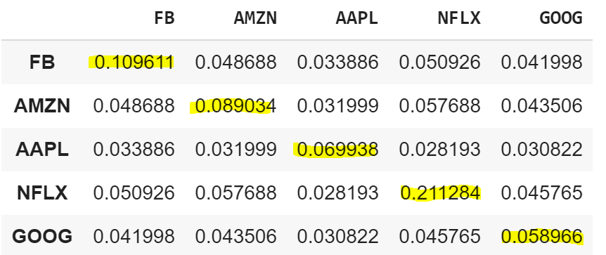
Now calculate and show the portfolio variance using the formula :Expected portfolio variance= WT * (Covariance Matrix) * W
port_variance = np.dot(weights.T, np.dot(cov_matrix_annual, weights))port_variance![]()
Now calculate and show the portfolio volatility using the formula :Expected portfolio volatility= SQRT (WT * (Covariance Matrix) * W)
![]()
Don?t forget the volatility (standard deviation) is just the square root of the variance.
port_volatility = np.sqrt(port_variance)port_volatility![]()
Last but least not I?m going to show and calculate the portfolio annual simple return.
portfolioSimpleAnnualReturn = np.sum(returns.mean()*weights) * 252portfolioSimpleAnnualReturn![]()
Show the expected annual return, volatility or risk, and variance.
percent_var = str(round(port_variance, 2) * 100) + ‘%’percent_vols = str(round(port_volatility, 2) * 100) + ‘%’percent_ret = str(round(portfolioSimpleAnnualReturn, 2)*100)+’%’print(“Expected annual return : “+ percent_ret)print(‘Annual volatility/standard deviation/risk : ‘+percent_vols)print(‘Annual variance : ‘+percent_var)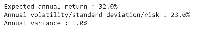
So, now I can see the expected annual return on the investments which is 32% and the amount of risk for this portfolio which is 23%, but can I do better ? I think I can.
Optimize The Portfolio
It?s now time to optimize this portfolio, meaning I want to optimize for the maximum return with the least amount of risk . Luckily their is a very nice package that can help with this created by Robert Ansrew Martin.
I will install the package that he created called pyportfolioopt.
pip install PyPortfolioOpt
Next, I will import the necessary libraries.
from pypfopt.efficient_frontier import EfficientFrontierfrom pypfopt import risk_modelsfrom pypfopt import expected_returns
Calculate the expected returns and the annualised sample covariance matrix of daily asset returns.
mu = expected_returns.mean_historical_return(df)#returns.mean() * 252S = risk_models.sample_cov(df) #Get the sample covariance matrix
Optimize for maximal Sharpe ration .
ef = EfficientFrontier(mu, S)weights = ef.max_sharpe() #Maximize the Sharpe ratio, and get the raw weightscleaned_weights = ef.clean_weights() print(cleaned_weights) #Note the weights may have some rounding error, meaning they may not add up exactly to 1 but should be closeef.portfolio_performance(verbose=True)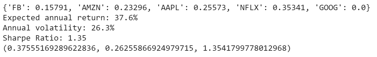
Now we see that we can optimize this portfolio by having about 15.791% of the portfolio in Facebook, 23.296% in Amazon , 25.573% in Apple, 35.341% in Netflix and 0% in Google.
Also I can see that the expected annual return has increased to 37.6% with this optimization and the annual volatility / risk is 26.3%. This optimized portfolio has a Sharpe ratio of 1.35 which is good. The numbers in the parenthesis at the bottom are the same three numbers I just mentioned in decimal form.
I want to get the discrete allocation of each share of the stock, meaning I want to know exactly how many of each stock I should buy given some amount that I am willing to put into this portfolio.
So, for example I am willing to put in $15,000 USD into this portfolio, and need to know how much of each stock I can purchase in the portfolio to give me the optimal results.
First I will install pulp.
pip install pulp
Now it?s time to get the discrete allocation of each stock.
from pypfopt.discrete_allocation import DiscreteAllocation, get_latest_priceslatest_prices = get_latest_prices(df)weights = cleaned_weights da = DiscreteAllocation(weights, latest_prices, total_portfolio_value=15000)allocation, leftover = da.lp_portfolio()print(“Discrete allocation:”, allocation)print(“Funds remaining: ${:.2f}”.format(leftover))
Alright ! Looks like I can buy 14 shares of Facebook, 2 shares of Amazon, 13 shares of Apple, and 16 shares of NetFlix for this optimized portfolio and still have about $51.67 USD leftover from my initial investment of $15,000 USD.
That?s it, we are done creating this program !
If you are also interested in reading more on Python one of the fastest growing programming languages that many companies and computer science departments use then I recommend you check out the book Learning Python written by Mark Lutz?s.
Learning Python
Thanks for reading this article I hope it?s helpful to you all! If you enjoyed this article and found it helpful please leave some claps to show your appreciation. Keep up the learning, and if you like Python, machine learning, mathematics, computer science, programming or algorithm analysis, please visit and subscribe to my YouTube channels (randerson112358 & compsci112358 ).

