Pivoting To Understand Quicksort [Part 1]

Pivoting to understand quicksort

Whether or not you?re new to sorting algorithms or familiar with some of them already, you?ve probably heard or read about today?s algorithm in some context or another. It?s reputation tends to precedes itself!

Quicksort ? the algorithm that we?ll be learning about this week and next week ? has been called the ?quickest? and ?most efficient? sorting algorithm by many people. In fact, in the handful of conversations that I?ve had with other programmers about sorting algorithms, quicksort almost always comes up as the best algorithm to use, and very few people ever seem to debate this fact.

But, what even is quicksort? Everyone says that it?s great and that we should use it, and that the problem of algorithms is pretty much figured out! Yet some of us ? myself included ? don?t even know what it is! Its time to change that. If we?re going to be true algorithmic masters, we?ve got to be well-informed on the in?s and out?s of this infamous algorithm!

It?s time to pivot, and finally understand how a quicksort algorithm works!

A quick study on quicksort basics

The quicksort algorithm is a particularly interesting one, and it took me awhile to wrap my head around it. We?re just going to focus on how it works and functions internally to start.

There is at least one thing about quicksort that we?re familiar with already ? we might not know it just yet. This algorithm does something that we?ve seen before: it breaks down a larger problem into smaller, subproblems. We might remember this concept from back when we were learning about merge sort! This is also known as a divide and conquer algorithm, which breaks down a problem into simpler versions of itself. Don?t worry if this isn?t obvious just yet; it will become more clear later on when we walk through the algorithm itself.

Okay, so what does this algorithm do, exactly? The quicksort algorithm is a sorting algorithm that sorts a collection by choosing a pivot point, and partitioning the collection around the pivot, so that elements smaller than the pivot are before it, and elements larger than the pivot are after it. It continues to choose a pivot point and break down the collection into single-element lists, before combing them back together to form one sorted list.

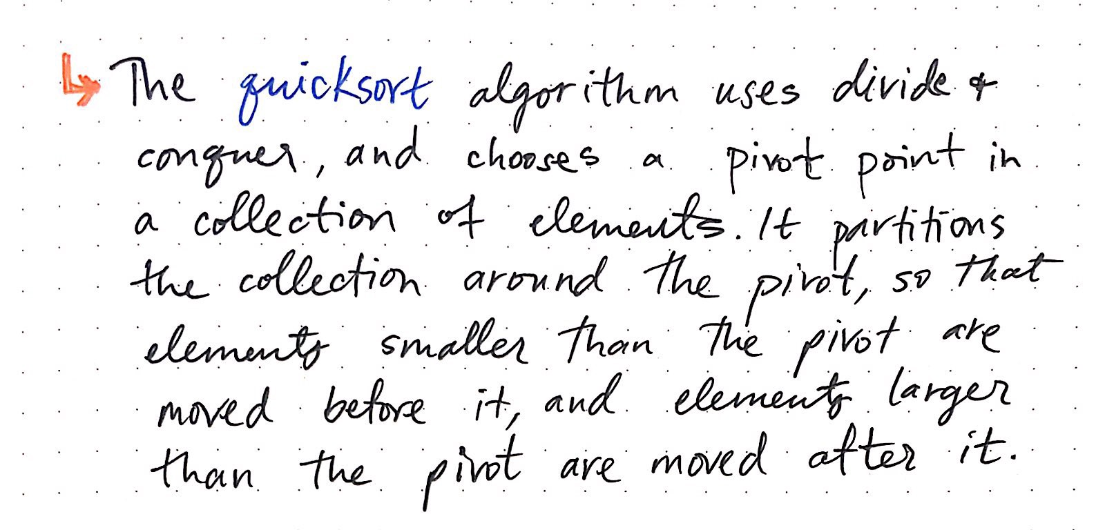Quicksort: a definition

If we read our definition again, we?ll see that there are really two core parts to how this algorithm functions.

1. First, quicksort determines something called a pivot, which is a somewhat arbitrary element in the collection.
2. Next, using the pivot point, it partitions (or divides) the larger unsorted collection into two, smaller lists. It uses some smart logic to decide how to do the partitioning: it moves all the elements smaller than the pivot to the left (before) the pivot element, and moves all the elements larger than the pivot to the right (after) the pivot element.

Wait, so what?s so smart about that? Why does partitioning the larger list so that elements smaller than the pivot are first and elements larger than the pivot are last matter? Well, let?s look at a simple example, without any real content just yet, and see if we determine what?s so clever about this algorithm.

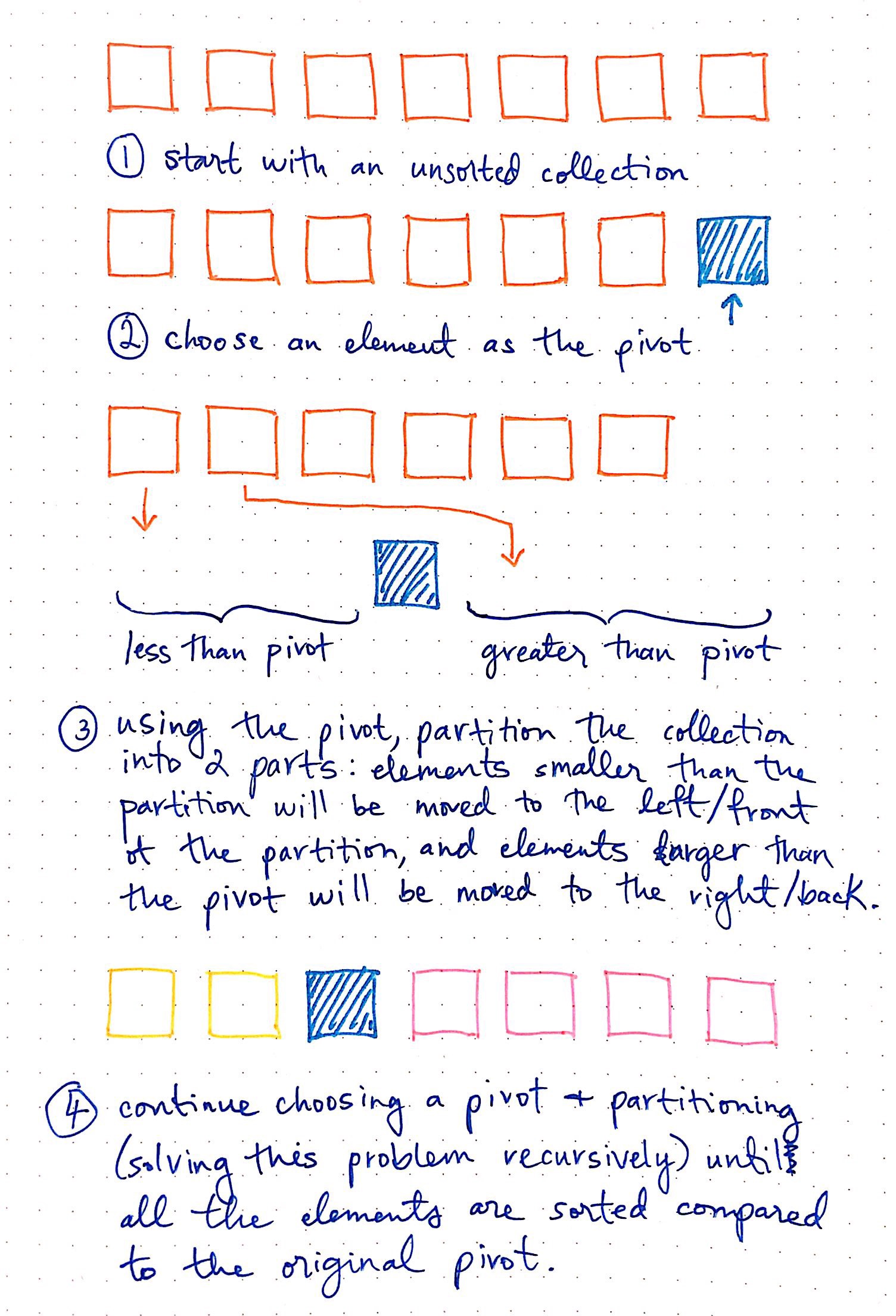
In the illustration below, we start off with an unsorted collection.

How quicksort works

We?ll choose the last element as the pivot for now. As it turns out, there are many different ways to choose a pivot element, and what you choose does matter ? but more on that in a bit. It?s pretty common to see implementations of quicksort with the last element as the pivot, so that?s what we?ll do here, too.

Okay, so we choose the last element as our pivot. Now, our quicksort algorithm will take all of the remaining, other elements, and reorder them so that all of the items smaller than our pivot are in front, or to the left of it, and all of the items larger than our pivot are behind, or to the right of it.

Since we know that quicksort is a divide and conquer algorithm, we also know that it?s going to implement the exact same logic that we just saw on the two partitioned sublists! In other words, it?s going to employ recursion here: it will choose a pivot element for each of the two sublists, and then divide each sublists into it?s own sublist, with two halves: a half that contains all the elements smaller than the pivot, and another half that contains all the elements larger than the pivot. It?ll continue calling itself upon itself recursively until it has only one element in each list ? remember than one element in a list is, by definition, considered sorted.

So, why is this powerful? Well, let?s take a closer look at the two partitions that we started off with here. The left partition, marked in yellow, represents all the items smaller than the pivot. The right partition, marked in pink, represents all the items greater than the pivot.

Even though the list isn?t completely sorted yet, we know that the items are in the correct order in relation to the pivot. This means that we never have to compare elements on the left side of the partition to elements on the right side of the partition. We already know they are in their correct spots in relation to the pivot.

Now that we understand how quicksort is clever about partitioning, it?s probably good to mention how it chooses a pivot ? or at least, how it ought to choose a pivot. Earlier, we learned that the pivot is a somewhat arbitrary element in the collection. The pivot element should be slightly random, but what we choose as the pivot is super important!

As we learn more about quicksort algorithms, we?ll see that different implementations will determine a pivot element in varying ways. There is not right or wrong element for a pivot, per se. However, there are a few things to keep in mind.

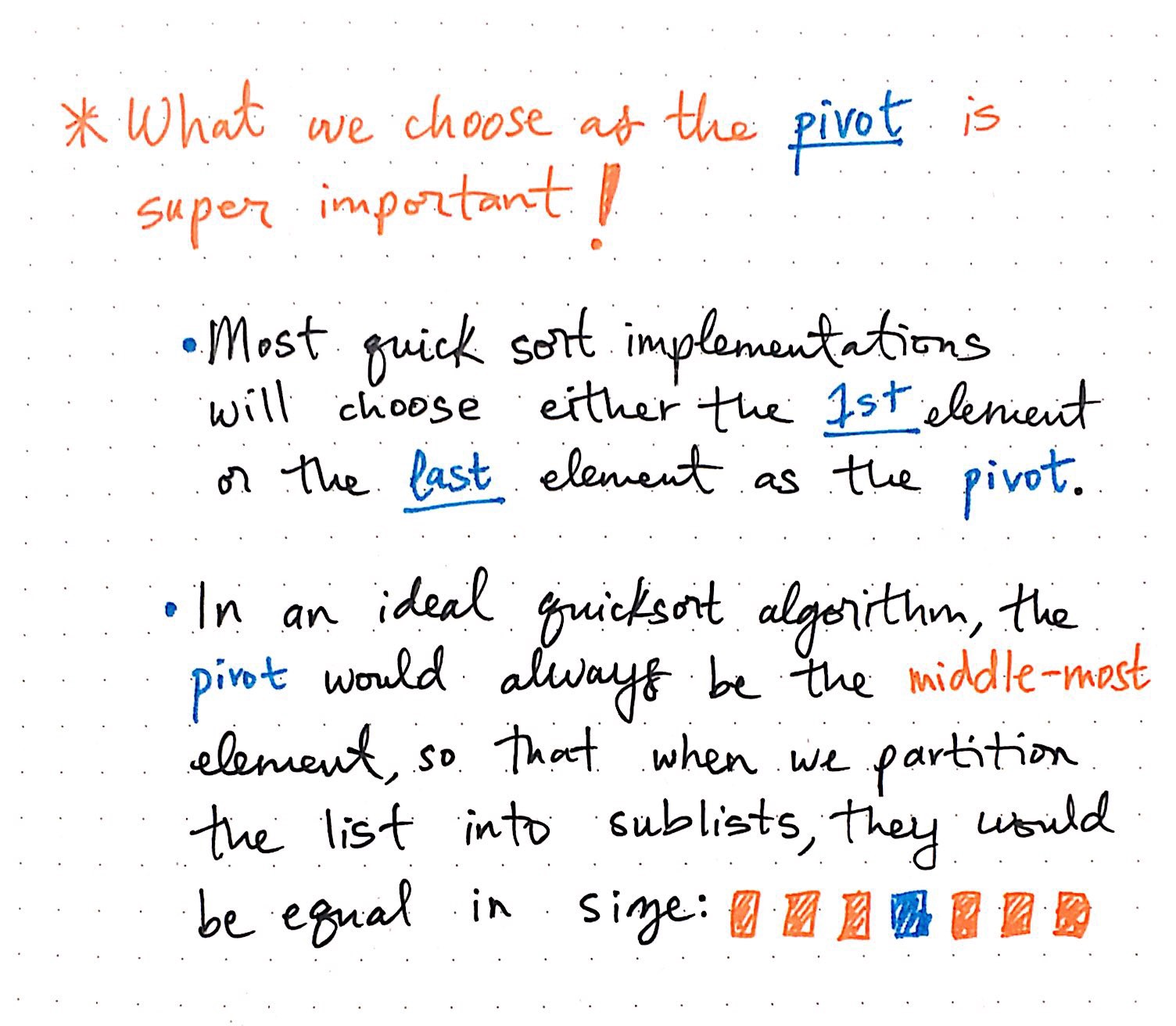What we choose as a pivot is important!

A quicksort algorithm should always aim to choose the middle-most element as its pivot. Some algorithms will literally select the center-most item as the pivot, while others will select the first or the last element. But when we say ?middle-most? element, what we mean is an element at the median of the entire unsorted collection. This ends up being super crucial because we want the two partitioned halves ? the elements smaller than the pivot and the elements larger than the pivot ? to be mostly equal. If they?re unequal or lopsided, we can run into some big problems!

We?ll get more into why this is important next week; for now, just know that how we choose the pivot is important, but it doesn?t necessarily have to be one element in particular.

Making quick work of quicksort

Now that we?re a little more well-versed in the theory behind how quicksort works, it?s time for us to see it in action! We?ll do this by walking through how quicksort would sort a small collection of numbers that might look something like this: [9, 12, 9, 2, 17, 1, 6].

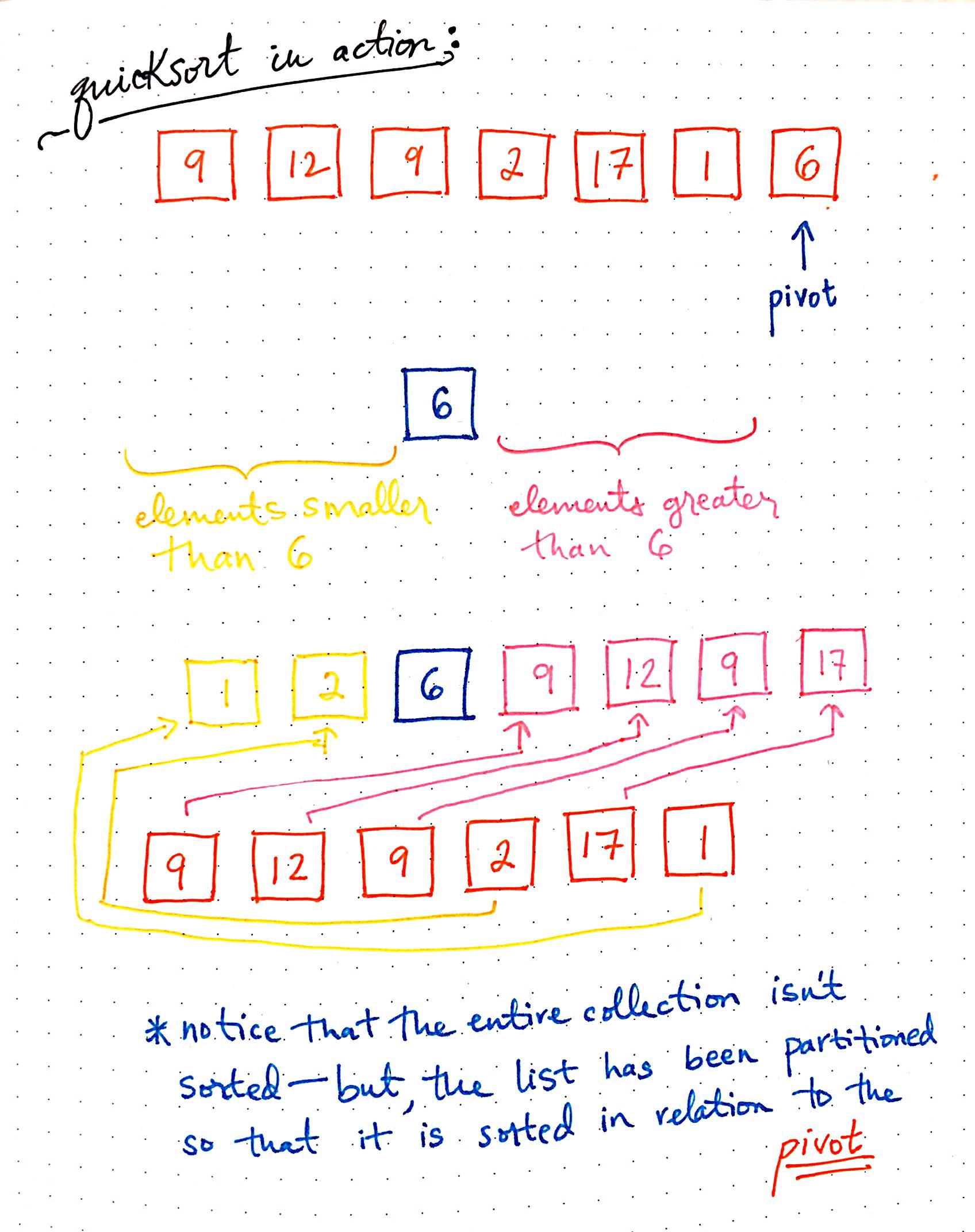Quick sort in action: part 1.

We?ll stick with what we?ve been doing so far and choose the last element as our pivot. In this case, the last element is 6, so that will be our pivot element.

In the example shown here, we?re going to move the remaining items around so that everything smaller than the element 6 is to the left of it, and everything larger than 6 is to the right of it.

For example, the first element is 9, which we know is larger than 6. So, it is moved to the right partition. The same goes for the next few elements within our unsorted list: 12 and 9. However, 2 is smaller than 6, so it is moved to the left partition.

Notice that, once we?re done moving all the elements around in relation to the pivot, we?re still not done! The entire collection hasn?t been sorted in relation to all the elements; however, we do know that the collection has been sorted in relation to the pivot element. This is helpful because we won?t need to compare elements in the left partition to elements in the right partition, which will save us some time down the road.

So, if we?re not done, what do we need to do next? Well, quicksort is a divide and conquer algorithm, which means that its designed to use the same solution on smaller subproblems. In other words, we can recursively take the exact same steps we did just now and apply them to the left and right partitions that still need to be sorted.

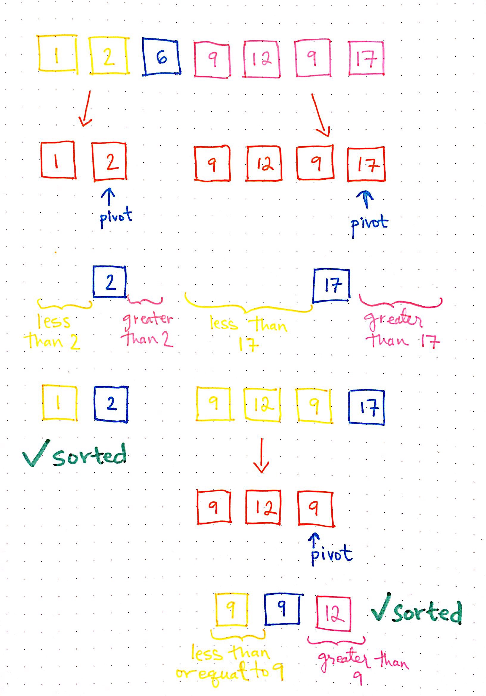Quick sort in action: part 2

Let?s see what that would look like.

In the second part of this walkthrough of quicksort, we will apply the same steps to the left and right partitions. Looking at the illustration shown here, we can see that we?re again, choosing the last element of both sublists as their respective pivot elements. For the left sublist, the partition is 2, and for the right sublist, the partition is 17.

Next, let?s look at the left sublist. There?s only one element in this list aside from the pivot: 1. It just so happens that 1 is already in the correct place: to the left of the pivot, 2, because it?s smaller than the pivot. So, this list is effectively sorted!

It?s a slightly different story for the right sublist, however. There are three elements in addition to the pivot: 9, 12, and 9. They?re all smaller than the pivot, 17, and they?re all to the left of the pivot. So, they?re in the correct partition given the pivot. But, we still need to sort them!

So, we?ll break those three elements down even further, into their own sublist, and recursively do the same work again: choose a pivot (9), and sort the remaining two items so that items greater than 9 are to the right, and items smaller or equal to 9 are to the left.

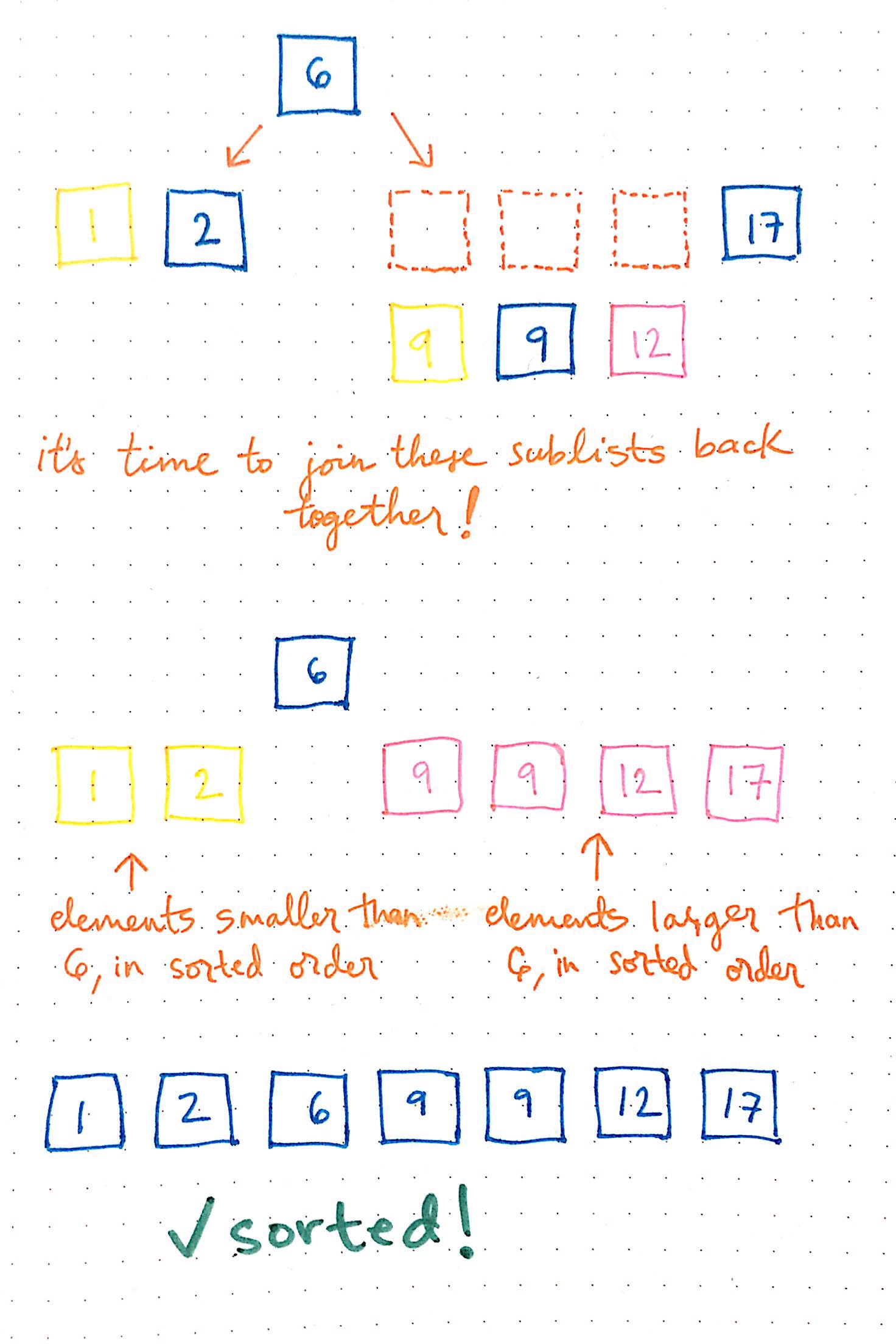Quick sort in action: part 3

Great! Now that all the sublists are sorted, there?s only one thing left to do: combine all the items together again, of course!

The last sublist that we sorted has these three elements in it: [9, 9, 12]. We?ll join this sublist with its parent sublist, so that it now contains these elements: [9, 9, 12, 17].

Rad! Now we can combine this sublist with the left partition sublist: [1, 2].

Notice how the two partitions here, left and right, both are sorted in comparison to the pivot, and in comparison to all the elements. In other words, all the items are in sorted order!

Notice how similar this is to what we saw with merge sort recently! We might be seeing some repeating patterns here, and they might even be a little reminiscent of binary search! We?ll see how these are related next week, when we look at the time complexity of quicksort at runtime. But for now, just noticing that there is some kind of pattern is enough.

Quick-fire swapping

We?ve walked through how quicksort runs, and how it uses recursion to implement the same algorithm again and again, on smaller and smaller sublists. But there?s one thing that still isn?t completely clear just yet: how does quicksort actually do the work of sorting elements into a left partition and a right partition? We know that it moves all the elements around and reorders them ? but how does this even happen?

One thought we might have here is that quicksort just creates a whole new array and copies over the elements in the correct order ? right? Well, not exactly. One of the many reasons that quicksort is a preferred algorithm is because it doesn?t take up a ton of extra space as it sorts! This means that it doesn?t have the luxury of being able to create a duplicated array, because that would take up a lot of space and memory.

Instead, this algorithm sorts elements in-place, which we might remember when we were first learning about sorting algorithms. This means that quicksor operates directly on the inputted data, and only needs a tiny bit of extra space in memory ? usually a constant amount of space.

So, if it doesn?t copy over elements into a new array?how does it sort them? The answer is: by swapping! This is probably the most complicated part of the quicksort algorithm; however, once we understand it, this algorithm makes a whole lot more sense.

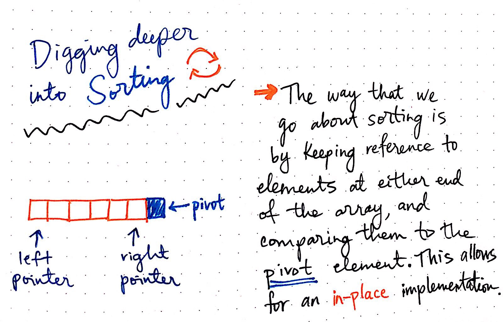Digging deeper into sorting

The way that quicksort goes about sorting elements into the respective partitions after choosing a pivot is by keep reference to elements at either end of the array or list, and then comparing the elements at those references to the pivot.

If the quicksort algorithm determines that two elements are out of order, it leans on its references to swap them into their correct place in the collection.

The basic steps to implementing the swap functionality can be a little complicated, so let?s look at the steps we?ll need to take before running through an example.

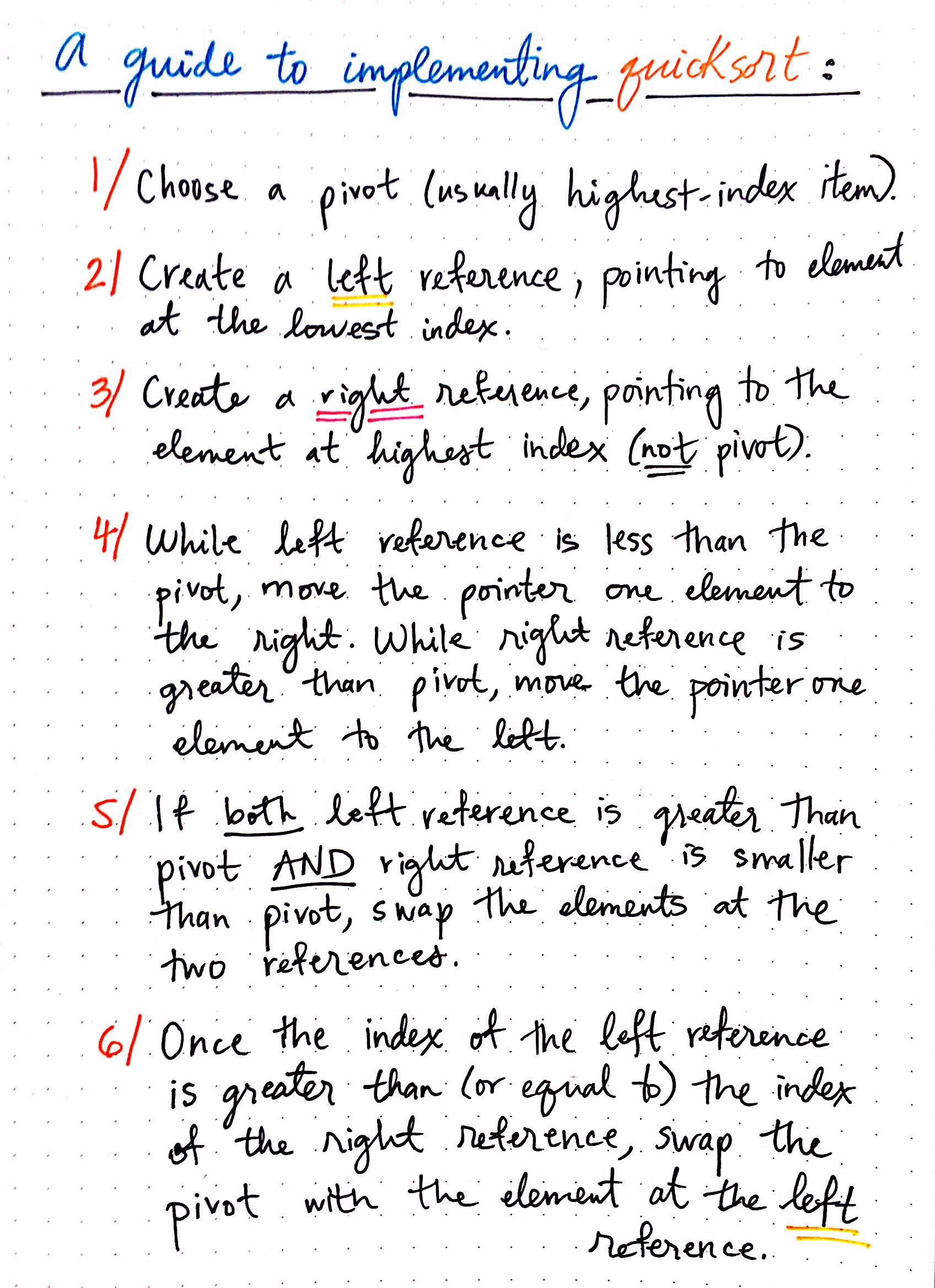A guide to implementing quicksort

First, we?ll want to choose a pivot (usually the last element)

Then, we?ll need to create a left reference to the lowest index (the first) element. And we?ll need to create a right reference to the highest index (the last) element ? excluding the pivot.

Next, we?ll need to compare left and right in relation to the pivot, independently.

For example, if the left reference is less than the pivot, then we know that it is smaller than the pivot, and will be in the correct partition. So, we can increment the left reference, moving one element over (to the right). The same goes for the right reference: if the element at the reference is greater than the pivot, we know it?ll be in the correct partition, so we can increment it one element over (to the left).

However ? if both the left reference is greater than the pivot and the right reference is smaller than the pivot, we know that we?ve stumbled upon two elements that are out of order.

In this situation, we can swap the two elements at the left reference and at the right reference so that they?re in the correct places ? and will subsequently end up in the correct partitions!

Once we finish going through all the elements, our left reference will ?pass? our right reference; in other words, the index of the left reference will be greater than the index of the right reference, meaning that we?ve finished sorting the two partitions. At this point, we can move the pivot into its correct place by swapping it with the item at the left reference. Another way to think about it is that the item at the left reference moves to the end of the right partition, and ends up becoming the new pivot for that sublist.

Let?s look at how quicksort does the work of swapping with an example.

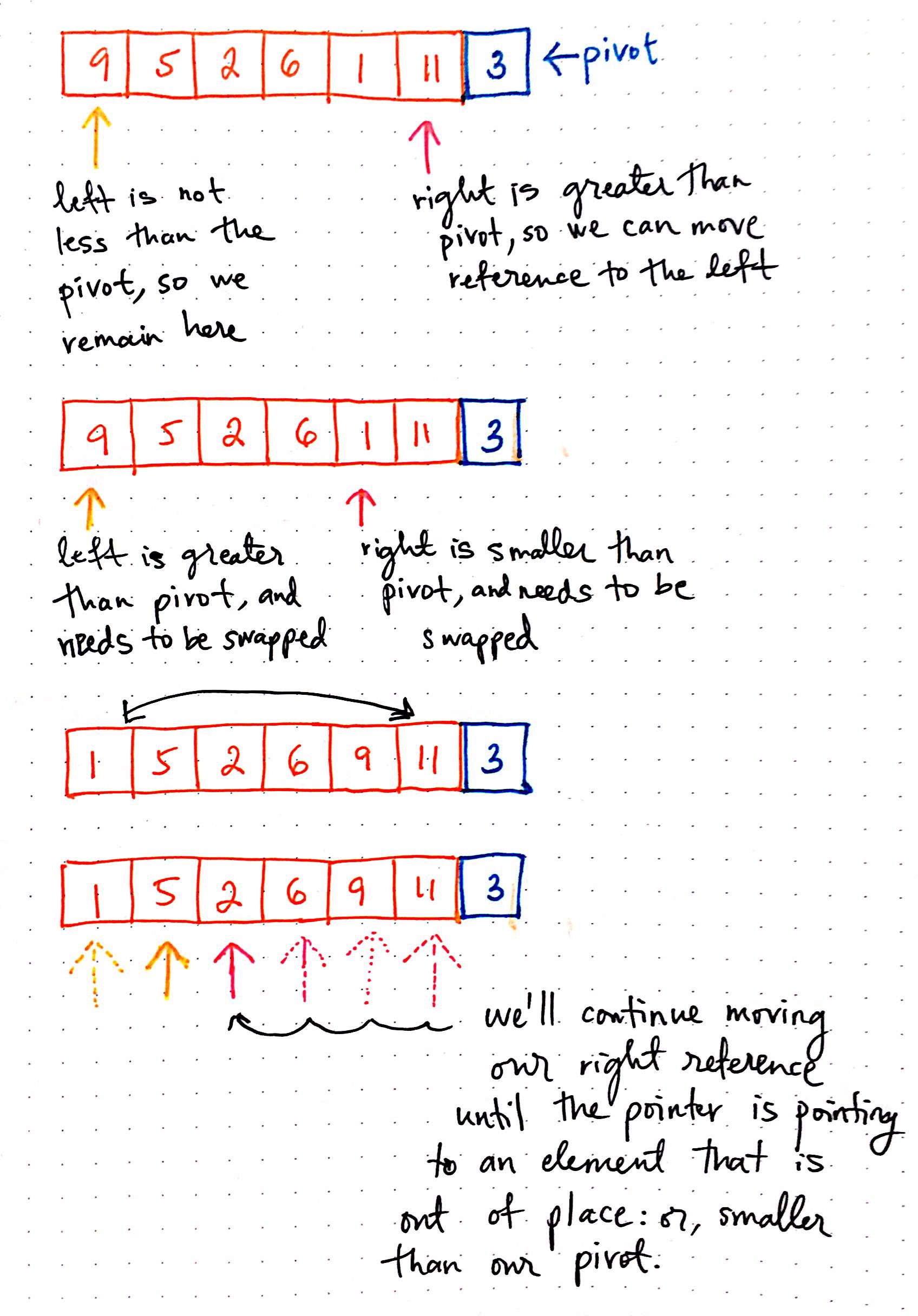How quicksort swaps: part 1

We start with the last item as our pivot: 3.We?ll create a left reference pointing to the first element, 9, and a right reference, pointing to the last element that is not the pivot, 11.

In our starting position, the left reference is not less than the pivot, which means that we need to swap it! However, the right reference is greater than the pivot, which means that it is in its correct place ? in other words, it?s going to be in the right partition, which is where it belongs.

So, we?ll increment the right pointer until we find an element that?s smaller than the pivot that we can swap with the left reference. As it turns out, when we move the right reference over one element, we come to a situation where the items can be swapped! The number 1 is smaller than 3, while 9 is greater than 3. So, we?ll swap these two elements.

We?ll continue moving our right and left references over until these pointers are at elements that are out of place.

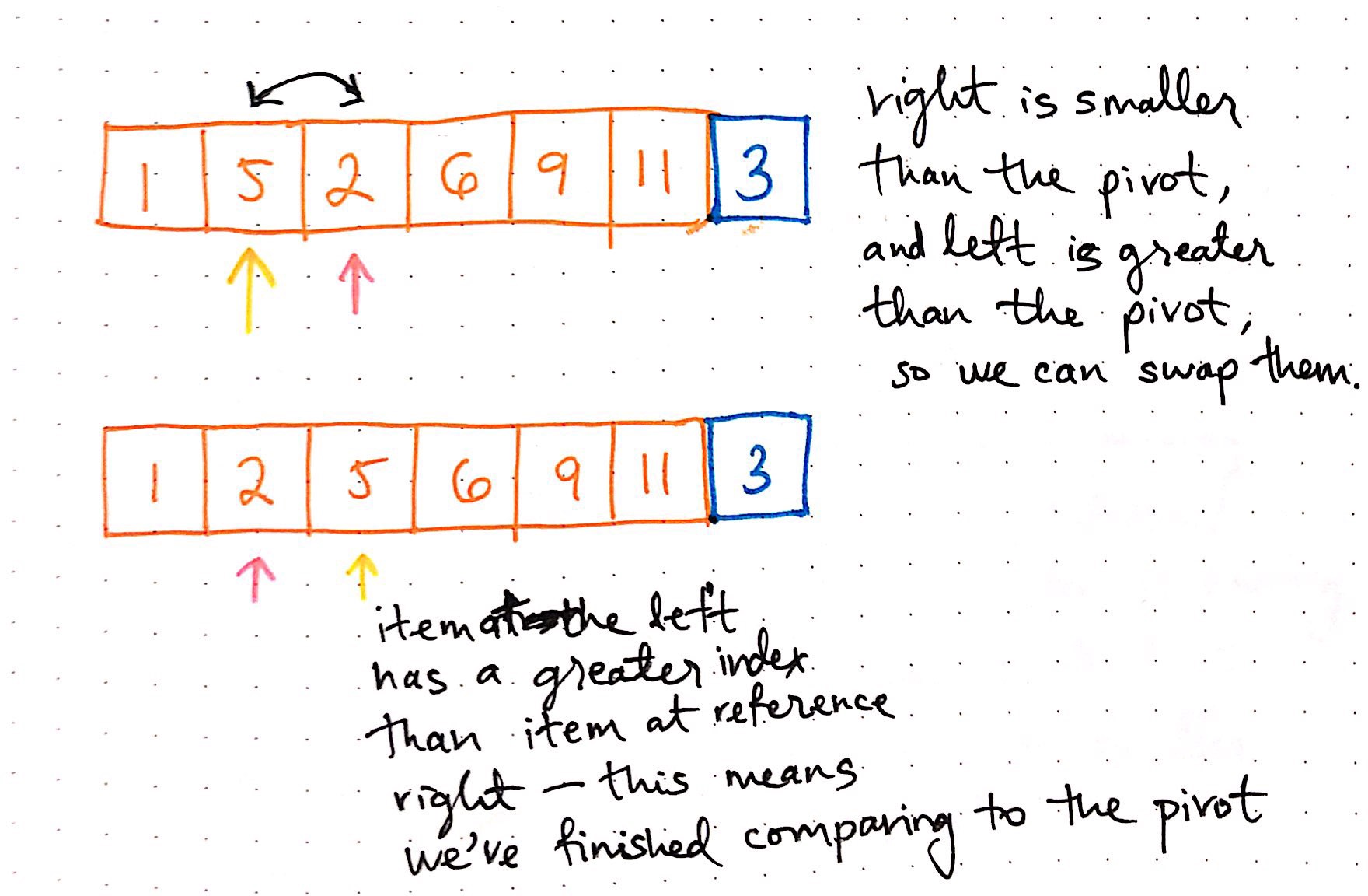How quicksort swaps: part 2

This doesn?t happen again until left is pointing at 5 and right is pointing at 2. We know that if left is greater than the pivot and right is less than the pivot, two elements are out of place. So, we?ll swap both 5 and 2.

Notice that now the left pointer has passed the right pointer ? that is to say, the item at left has a greater index than the item at right. This means that we?ve finished comparing all the elements to the pivot!

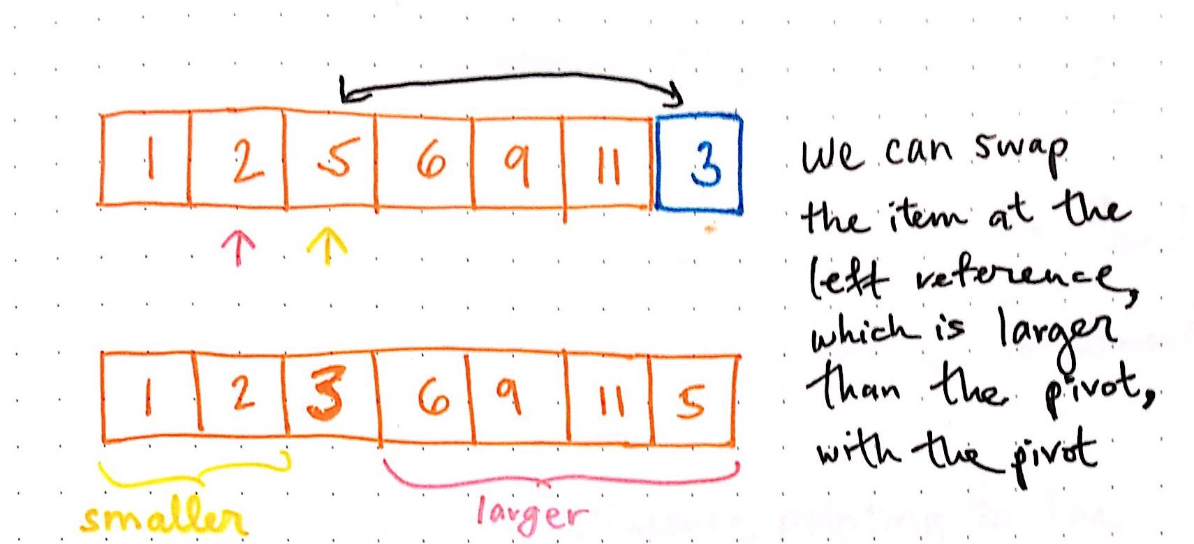How quicksort swaps: part 3

The last step now is to swap the item at the left reference with the pivot element. In this case, we?re swapping 5 and 3. Once we?ve done this, we can see that our two partitions are correctly divided! All the elements smaller than our pivot, 3, are to the left of it, and all the elements greater than our pivot are to the right! If we were to continue running quicksort, we?d divide these two partitions and invoke the quicksort algorithm upon the two sublists recursively.

The super cool thing is that the actual swap function itself isn?t super complicated on its own:

But, what it?s doing is pretty cool! It basically sorts elements within the context of the same array that they live in, and it does this in a mostly efficient way.

In part 2 of this series, we?ll implement this algorithm ourselves! We?ll also look at the runtime complexity of quicksort, when quicksort can go terribly wrong, and why it?s considered the most efficient sorting algorithm. Until then, I leave you with this cliffhanger!

Resources

Quicksort is heavily-used by various programming languages to implement their sorting algorithms as efficiently as possible. As it turns out, there are a lot of resources on this particular algorithm, and it can be a little overwhelming to sift through them all (it was for me, at least!). If you?re curious to learn more about quick sort, here are a few of my favorite places to start.

1. Quicksort algorithm, mycodeschool
2. Sorting Algorithms: QuickSort, Professor Lydia Sinapova
3. Quick Sort, Computerphile
4. Data Structure and Algorithms ? Quick Sort, Tutorialspoint
5. QuickSort, GeeksForGeeks
6. Quick Sort in 4 Minutes, Michael Sambol