Normalizing Numerical Values in Excel

sheetsFollowJan 9 5 min read

Before running any sort of analysis, a lot of the times we need to normalize numerical values to fit a certain range or distribution.

This is just for the thumbnail. Please ignore

This process is generally known as normalization. However, it can also be called standardization or transformation. The three terms are actually different:

Normalization ? Changing the original numerical values to fit within a certain range.

• For e.g., you want to modify test scores that could be between 0?100 to be within the range 0?1.
• You might want to normalize when you have multiple variables with differing ranges. For e.g., if you have variables Test Score 1 and Test Score 2 where Test Score 1 was out of 100 while Test Score 2 was out of 40.

The formula for normalizing a value x that comes from a range (y, z) between a range (a, b):

X_normalized = (b – a) * [ (x – y) / (z – y) ] + a

Standardization ? Changing the original numerical values to fit within a distribution that has a mean of 0 and standard deviation of 1. The standardize values are also called z-scores, which you can then use to see how far a given value is from a certain mean.

• For e.g., you have stock market data for 30 days that has a mean of 550 and standard deviation of 3 but you want to standardize the data so the mean is 0 and standard deviation is 1.
• You might want to standardize to detect outliers in a given range or to compare two disparate sets of data. For ex: if you have stock market data for Company A with the above mean and standard deviation and then you have stock market data for Company B that has mean of 750 and standard deviation of 5.

The formula for standardizing a value x from range (y, z):

X_standardized = (x – mean_of_range) / standard_deviation_range

Transformation ? Changing the original numerical values to fit a specific distribution that your data analysis needs.

• This is a more complex topic that we will cover in a separate blog post.
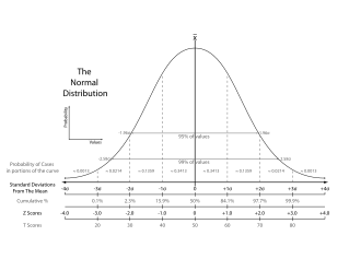
• Meanwhile, if you are interested you can read more about transforming data to a normal (gaussian) distribution, also known as a bell curve, by using the Box Cox transform. This is just one of many other transforms available

How To Normalize Values in Excel

First, let?s see what kind of values we will be normalizing. These are test scores for 39 students in an Intro to Computer Science class on Test 1 and Test 2. Test 1 was scored out of 50 while Test 2 was scored out of 40.

Our dataset originally had two columns Test 1 and Test 2. I have also added Test 1 Norm and Test 2 Norm. You can download the full file with the normalized scores and formulas here.

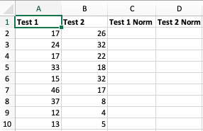Test Scores for 9 out of the 39 students. We have added the last two columns to store our results

The reason we are normalizing is we want to create a predictive model that can take some variables such as student household income, residential area etc. and accurately predict the students test scores on future tests.

We will be normalizing both scores between 1?5 simply because we will have some integer values and it will be easier for people to share their scores. You can substitute the min and max of your range in the formula below.

Once again the formula for normalizing is:

X_normalized = (b – a) * [ (x – y) / (z – y) ] + a

First we are going to normalize Test 1 scores. So in cell C2, we will enter the following Excel formula

= (5 ? 1) * ( (A2 ? MIN($A$2:$A$40)) / (MAX($A$2:$A$40) ? MIN($A$2:$A$40)) ) + 1

Let?s walk through the formula real quick:

1. b is the max value of the range we want to normalize to, which in this case is 5
2. a is the min value of the range we want to normalize to, which in this case is 1
3. Since we are starting from A2, we put that as the first x value. When we drag down the formula the A2 will get replaced with the corresponding input x value
4. y is the minimum of our input range. We determine the minimum of the range by the MIN formula in Excel. We give the range with the dollar signs because we don?t want those variables to be changed as we drag the formula down. So our range is given $A$2:$A$40. The 40 is because we have 39 students, we would change this to our max row whatever that might be.
5. z is the maximum of our input range. We determine the maximum of the range by the MAX formula in Excel. We give the same range as above.
6. Finally, we add 1 to everything as that is the minimum of our normalized range

Entering and dragging this down in the Test 1 Norm column gives us the following normalized scores for the first 10 students for Test 1

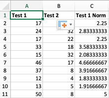As you can see the perfect score of 50 got normalized to 5

We will do the same for Test 2 except the x value in the Excel formula will change to B2 to correspond to the Test 2 score and the range will change to $B$2:$B$40

= (5 ? 1) * ( (B2 ? MIN($B$2:$B$40)) / (MAX($B$2:$B$40) ? MIN($B$2:$B$40))) + 1

Entering and dragging this formula down in the Test 2 Norm column gives us the following normalized scores for the first 10 students for Test 2

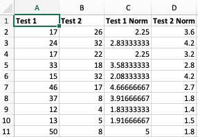
As you can see it is now waayyyy easier to compare scores. Nothing is too dramatic in these 10 scores but you can judge how much better someone did way easier.

That?s it! Go forth and normalize away!