Neural Style Transfer: Creating Art with Deep Learning using tf.keras and eager execution

By Raymond Yuan, Software Engineering Intern

In this tutorial, we will learn how to use deep learning to compose images in the style of another image (ever wish you could paint like Picasso or Van Gogh?). This is known as neural style transfer! This is a technique outlined in Leon A. Gatys? paper, A Neural Algorithm of Artistic Style, which is a great read, and you should definitely check it out.

Neural style transfer is an optimization technique used to take three images, a content image, a style reference image (such as an artwork by a famous painter), and the input image you want to style ? and blend them together such that the input image is transformed to look like the content image, but ?painted? in the style of the style image.

For example, let?s take an image of this turtle and Katsushika Hokusai?s The Great Wave off Kanagawa:

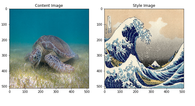Image of Green Sea Turtle by P. Lindgren, from Wikimedia Commons

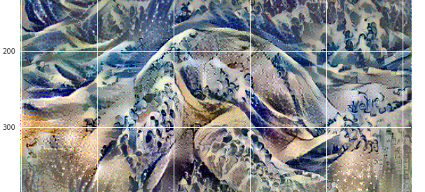
Now how would it look like if Hokusai decided to add the texture or style of his waves to the image of the turtle? Something like this?

Is this magic or just deep learning? Fortunately, this doesn?t involve any magic: style transfer is a fun and interesting technique that showcases the capabilities and internal representations of neural networks.

The principle of neural style transfer is to define two distance functions, one that describes how different the content of two images are, Lcontent, and one that describes the difference between the two images in terms of their style, Lstyle. Then, given three images, a desired style image, a desired content image, and the input image (initialized with the content image), we try to transform the input image to minimize the content distance with the content image and its style distance with the style image.

In summary, we?ll take the base input image, a content image that we want to match, and the style image that we want to match. We?ll transform the base input image by minimizing the content and style distances (losses) with backpropagation, creating an image that matches the content of the content image and the style of the style image.

Specific concepts that will be covered:

In the process, we will build practical experience and develop intuition around the following concepts:

• Eager Execution ? use TensorFlow?s imperative programming environment that evaluates operations immediately
• Learn more about eager execution
• See it in action (many of the tutorials are runnable in Colaboratory)
• Using Functional API to define a model ? we?ll build a subset of our model that will give us access to the necessary intermediate activations using the Functional API
• Leveraging feature maps of a pretrained model ? Learn how to use pretrained models and their feature maps
• Create custom training loops ? we?ll examine how to set up an optimizer to minimize a given loss with respect to input parameters

We will follow the general steps to perform style transfer:

1. Visualize data
2. Basic Preprocessing/preparing our data
3. Set up loss functions
4. Create model
5. Optimize for loss function

Audience: This post is geared towards intermediate users who are comfortable with basic machine learning concepts. To get the most out of this post, you should:

• Read Gatys? paper ? we?ll explain along the way, but the paper will provide a more thorough understanding of the task
• Understand gradient descent

Time Estimated: 60 min

Code:

You can find the complete code for this article at this link. If you?d like to step through this example, you can find the colab here.

Implementation

We?ll begin by enabling eager execution. Eager execution allows us to work through this technique in the clearest and most readable way.

Image of Green Sea Turtle -By P .Lindgren from Wikimedia Commons and Image of The Great Wave Off Kanagawa from by Katsushika Hokusai Public Domain

Define content and style representations

In order to get both the content and style representations of our image, we will look at some intermediate layers within our model. Intermediate layers represent feature maps that become increasingly higher ordered as you go deeper. In this case, we are using the network architecture VGG19, a pretrained image classification network. These intermediate layers are necessary to define the representation of content and style from our images. For an input image, we will try to match the corresponding style and content target representations at these intermediate layers.

Why intermediate layers?

You may be wondering why these intermediate outputs within our pretrained image classification network allow us to define style and content representations. At a high level, this phenomenon can be explained by the fact that in order for a network to perform image classification (which our network has been trained to do), it must understand the image. This involves taking the raw image as input pixels and building an internal representation through transformations that turn the raw image pixels into a complex understanding of the features present within the image. This is also partly why convolutional neural networks are able to generalize well: they?re able to capture the invariances and defining features within classes (e.g., cats vs. dogs) that are agnostic to background noise and other nuisances. Thus, somewhere between where the raw image is fed in and the classification label is output, the model serves as a complex feature extractor; hence by accessing intermediate layers, we?re able to describe the content and style of input images.

Specifically we?ll pull out these intermediate layers from our network:

Model

In this case, we load VGG19, and feed in our input tensor to the model. This will allow us to extract the feature maps (and subsequently the content and style representations) of the content, style, and generated images.

We use VGG19, as suggested in the paper. In addition, since VGG19 is a relatively simple model (compared with ResNet, Inception, etc) the feature maps actually work better for style transfer.

In order to access the intermediate layers corresponding to our style and content feature maps, we get the corresponding outputs by using the Keras Functional API to define our model with the desired output activations.

With the Functional API, defining a model simply involves defining the input and output: model = Model(inputs, outputs).

In the above code snippet, we?ll load our pretrained image classification network. Then we grab the layers of interest as we defined earlier. Then we define a Model by setting the model?s inputs to an image and the outputs to the outputs of the style and content layers. In other words, we created a model that will take an input image and output the content and style intermediate layers!

Define and create our loss functions (content and style distances)

Content Loss:

Our content loss definition is actually quite simple. We?ll pass the network both the desired content image and our base input image. This will return the intermediate layer outputs (from the layers defined above) from our model. Then we simply take the euclidean distance between the two intermediate representations of those images.

More formally, content loss is a function that describes the distance of content from our input image x and our content image, p . Let C?? be a pre-trained deep convolutional neural network. Again, in this case we use VGG19. Let X be any image, then C??(x) is the network fed by X. Let F???(x)? C??(x)and P???(x) ? C??(x) describe the respective intermediate feature representation of the network with inputs x and p at layer l . Then we describe the content distance (loss) formally as:

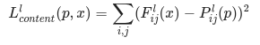
We perform backpropagation in the usual way such that we minimize this content loss. We thus change the initial image until it generates a similar response in a certain layer (defined in content_layer) as the original content image.

This can be implemented quite simply. Again it will take as input the feature maps at a layer L in a network fed by x, our input image, and p, our content image, and return the content distance.

Style Loss:

Computing style loss is a bit more involved, but follows the same principle, this time feeding our network the base input image and the style image. However, instead of comparing the raw intermediate outputs of the base input image and the style image, we instead compare the Gram matrices of the two outputs.

Mathematically, we describe the style loss of the base input image, x, and the style image, a, as the distance between the style representation (the gram matrices) of these images. We describe the style representation of an image as the correlation between different filter responses given by the Gram matrix G?, where G??? is the inner product between the vectorized feature map i and j in layer l. We can see that G??? generated over the feature map for a given image represents the correlation between feature maps i and j.

To generate a style for our base input image, we perform gradient descent from the content image to transform it into an image that matches the style representation of the original image. We do so by minimizing the mean squared distance between the feature correlation map of the style image and the input image. The contribution of each layer to the total style loss is described by

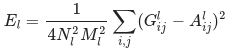
where G??? and A??? are the respective style representation in layer l of input image x and style image a. Nl describes the number of feature maps, each of size Ml=height?width. Thus, the total style loss across each layer is

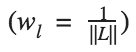
where we weight the contribution of each layer?s loss by some factor wl. In our case, we weight each layer equally:

This is implemented simply:

Run Gradient Descent

If you aren?t familiar with gradient descent/backpropagation or need a refresher, you should definitely check out this resource.

In this case, we use the Adam optimizer in order to minimize our loss. We iteratively update our output image such that it minimizes our loss: we don?t update the weights associated with our network, but instead we train our input image to minimize loss. In order to do this, we must know how we calculate our loss and gradients. Note that the L-BFGS optimizer, which if you are familiar with this algorithm is recommended, but isn?t used in this tutorial because a primary motivation behind this tutorial was to illustrate best practices with eager execution. By using Adam, we can demonstrate the autograd/gradient tape functionality with custom training loops.

Compute the loss and gradients

We?ll define a little helper function that will load our content and style image, feed them forward through our network, which will then output the content and style feature representations from our model.

Here we use tf.GradientTape to compute the gradient. It allows us to take advantage of the automatic differentiation available by tracing operations for computing the gradient later. It records the operations during the forward pass and then is able to compute the gradient of our loss function with respect to our input image for the backwards pass.

Then computing the gradients is easy:

Apply and run the style transfer process

And to actually perform the style transfer:

And that?s it!

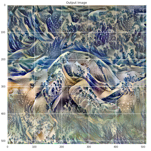
Let?s run it on our image of the turtle and Hokusai?s The Great Wave off Kanagawa:

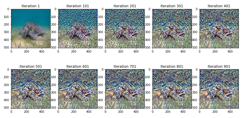
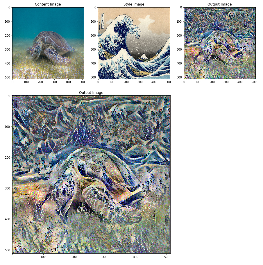Image of Green Sea Turtle by P.Lindgren [CC BY-SA 3.0 (https://creativecommons.org/licenses/by-sa/3.0)], from Wikimedia Common

Watch the iterative process over time:

Here are some other cool examples of what neural style transfer can do. Check it out!

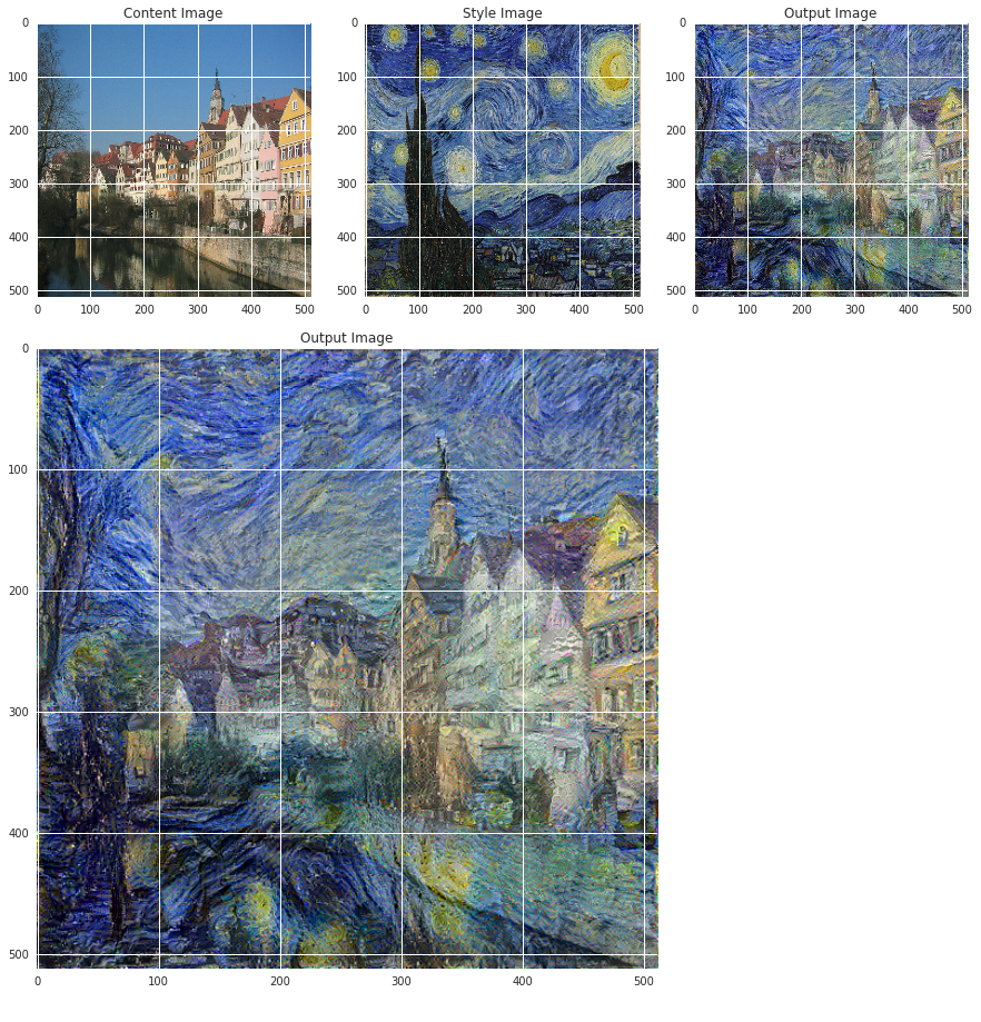Image of Tuebingen ? Photo By: Andreas Praefcke [GFDL (http://www.gnu.org/copyleft/fdl.html) or CC BY 3.0 (https://creativecommons.org/licenses/by/3.0)], from Wikimedia Commons and Image of Starry Night by Vincent van Gogh Public domain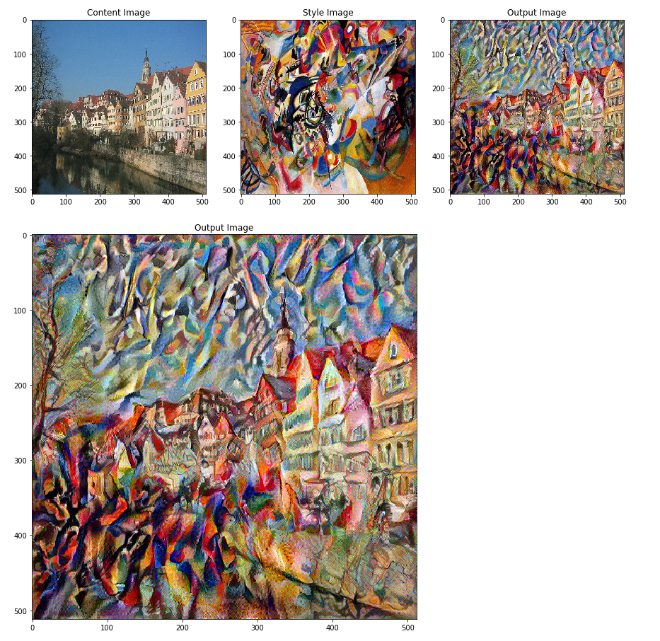Image of Tuebingen ? Photo By: Andreas Praefcke [GFDL (http://www.gnu.org/copyleft/fdl.html) or CC BY 3.0 (https://creativecommons.org/licenses/by/3.0)], from Wikimedia Commons and Image of Composition 7 by Vassily Kandinsky, Public Domain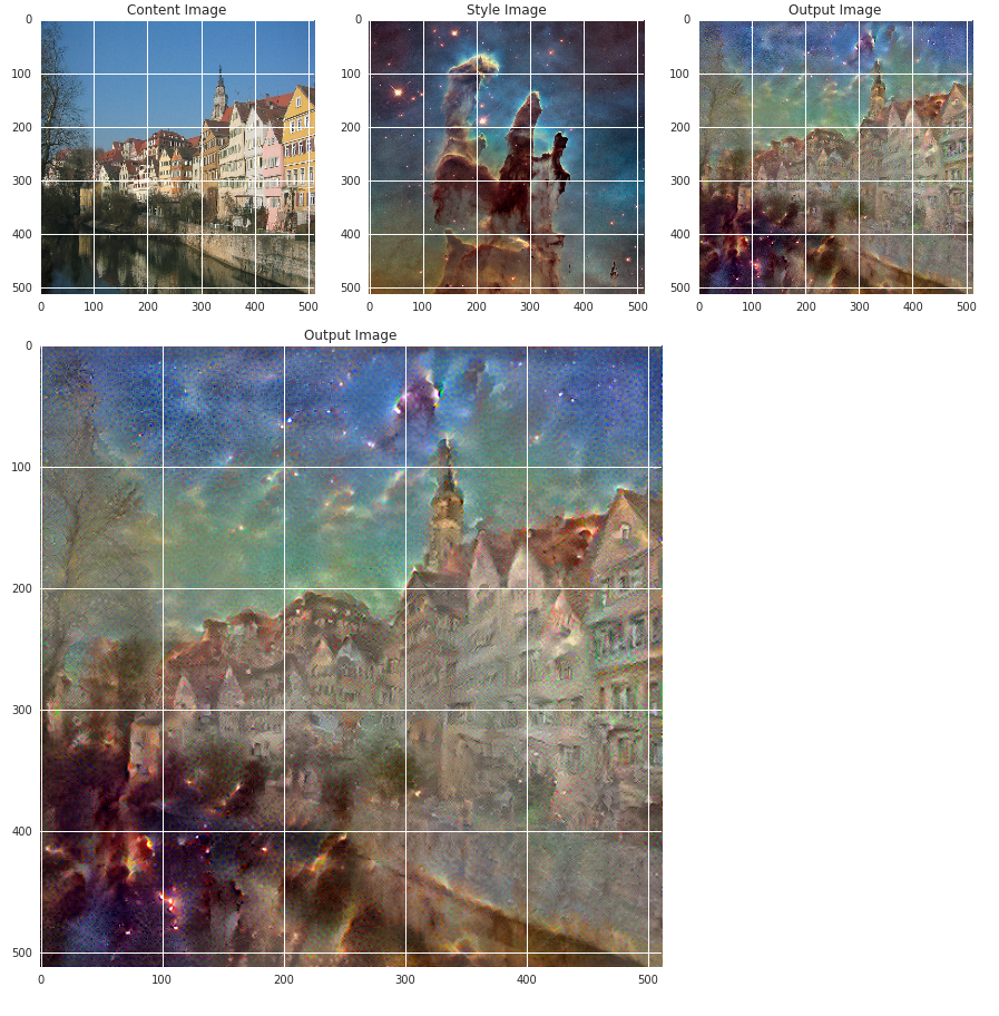Image of Tuebingen ? Photo By: Andreas Praefcke [GFDL (http://www.gnu.org/copyleft/fdl.html) or CC BY 3.0 (https://creativecommons.org/licenses/by/3.0)], from Wikimedia Commons and Image of Pillars of Creation by NASA, ESA, and the Hubble Heritage Team, Public Domain

Try out your own images!

Key Takeaways

What we covered:

• We built several different loss functions and used backpropagation to transform our input image in order to minimize these losses.
• In order to do this, we loaded in a pretrained model and used its learned feature maps to describe the content and style representation of our images.
• Our main loss functions were primarily computing the distance in terms of these different representations.
• We implemented this with a custom model and eager execution.
• We built our custom model with the Functional API.
• Eager execution allows us to dynamically work with tensors, using a natural python control flow.
• We manipulated tensors directly, which makes debugging and working with tensors easier.

We iteratively updated our image by applying our optimizers update rules using tf.gradient. The optimizer minimized the given losses with respect to our input image.