Missing data is a common problem in practical data analysis. They are simply observations that we intend to make but did not. In datasets, missing values could be represented as ???, ?nan?, ?N/A?, blank cell, or sometimes ?-999?, ?inf?, ?-inf?. The aim of this tutorial is to provide an introduction of missing data and describe some basic methods on how to handle them.
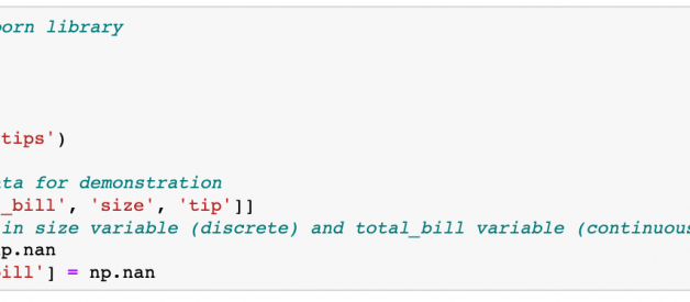
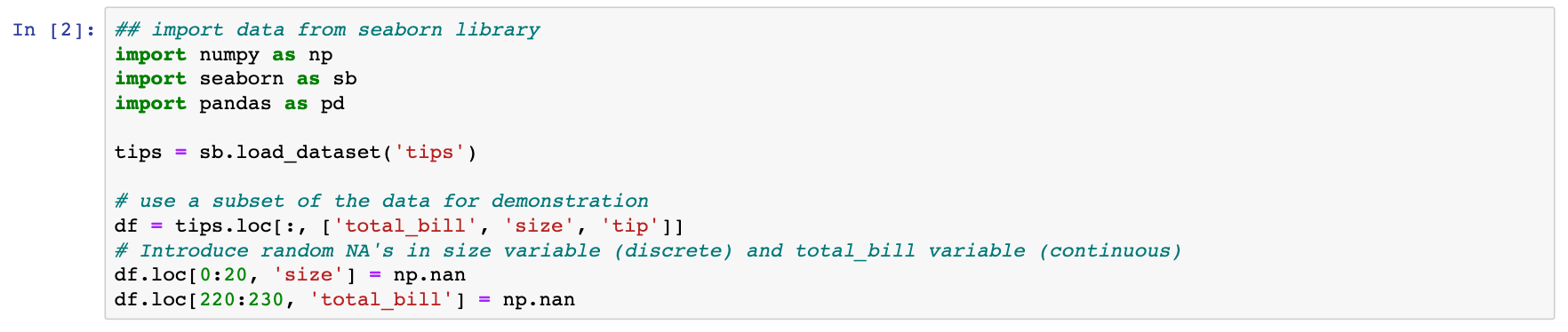
We use a simple dataset on tips from seaborn library for demonstration throughout the tutorial.
The study of missing data was formalized by Donald Rubin (see [6], [5]) with the concept of missing mechanism in which missing-data indicators are random variables and assigned a distribution. Missing data mechanism describes the underlying mechanism that generates missing data and can be categorized into three types ? missing completely at random (MCAR), missing at random (MAR), and missing not at random (MNAR). Informally speaking, MCAR means that the occurrence of missing values is completely at random, not related to any variable. MAR implies that the missingness only relate to the observed data and NMAR refers to the case that the missing values are related to both observed and unobserved variable and the missing mechanism cannot be ignored.
It is important to consider missing data mechanism when deciding how to deal with missing data. If the missing data mechanism is MCAR, some simple method may yield unbiased estimates but when the missing mechanism is NMAR, no method will likely uncover the truth unless additional information is unknown. We start our discussion with some simple methods.
Complete Case Analysis
As we can imagine, the simplest thing to do is to ignore the missing values. This approach is known as complete case analysis where we only consider observations where all variables are observed.
To drop entries with missing values in any column in pandas, we can use:

In general, this method should not be used unless the proportion of missing values is very small (<5%). Complete case analysis has the cost of having less data and the result is highly likely to be biased if the missing mechanism is not MCAR.
Besides complete case analysis, all other methods that we will talk about in this tutorial are all imputation methods. Imputation simply means that we replace the missing values with some guessed/estimated ones.
Mean, median, mode imputation
A simple guess of a missing value is the mean, median, or mode (most frequently appeared value) of that variable.
In pandas, .fillna can be used to replace NA?s with a specified value.

Regression imputation
Mean, median or mode imputation only look at the distribution of the values of the variable with missing entries. If we know there is a correlation between the missing value and other variables, we can often get better guesses by regressing the missing variable on other variables.
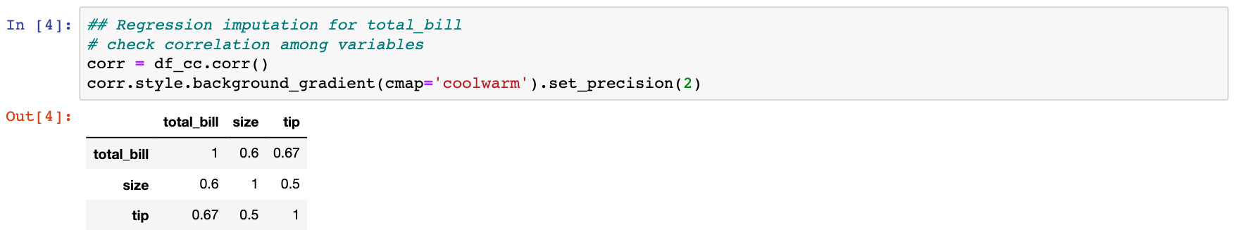
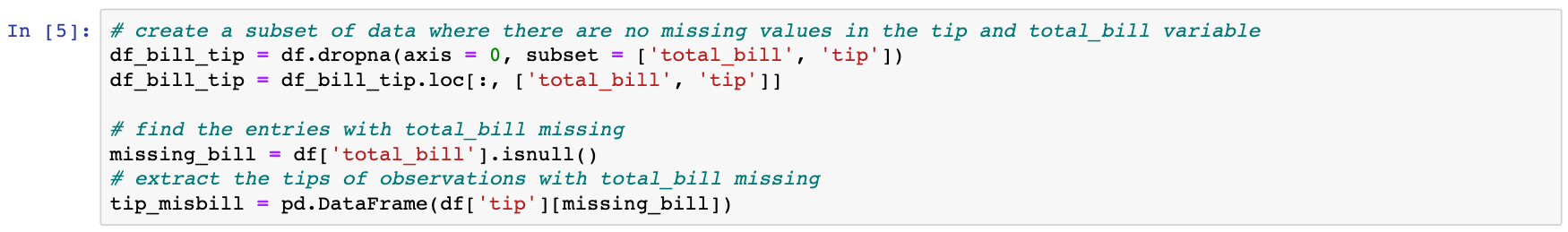
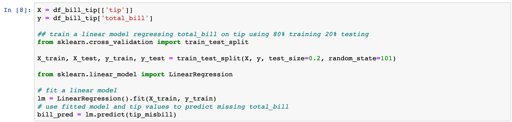
As we can see, in our example data, tip and total_bill have the highest correlation. Thus, we can use a simple linear model regressing total_bill on tip to fill the missing values in total_bill.
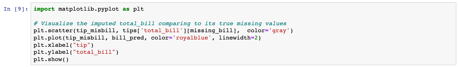
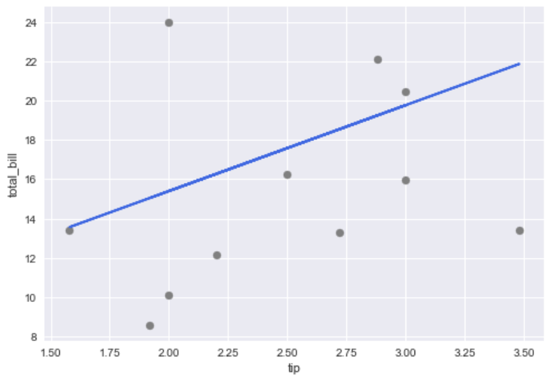
As we can see, the imputed total_bill from a simple linear model from tips does not exactly recover the truth but capture the general trend (and is better a single value imputation such as mean imputation). We can, of course, use more variables in the regression model to get better imputation.
Another way to improve regression imputation is the stochastic regression imputation, where a random error is added to the predicted value from the regression. For more on this, see chapter 1.3 of [6].
K-nearest neighbour (KNN) imputation
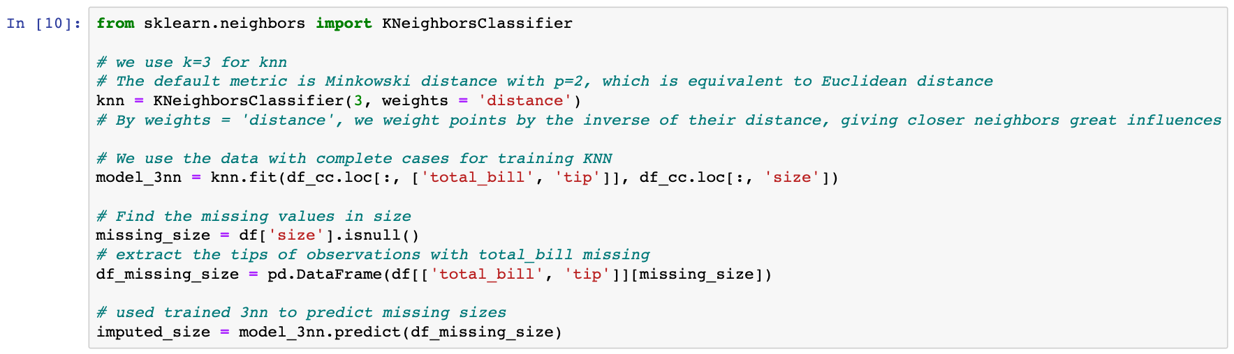
Besides model-based imputation like regression imputation, neighbour-based imputation can also be used. K-nearest neighbour (KNN) imputation is an example of neighbour-based imputation. For a discrete variable, KNN imputer uses the most frequent value among the k nearest neighbours and, for a continuous variable, use the mean or mode.
To use KNN for imputation, first, a KNN model is trained using complete data. For continuous data, commonly used distance metric include Euclidean, Mahapolnis, and Manhattan distance and, for discrete data, hamming distance is a frequent choice.
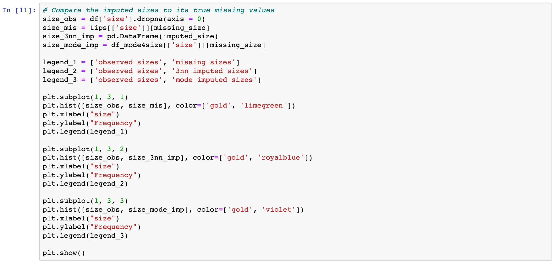
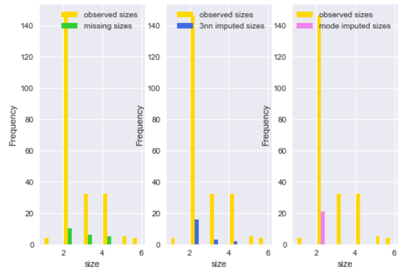
In the plot above, we compared the missing sizes and imputed sizes using both 3NN imputer and mode imputation. As we can see, KNN imputer gives much better imputation than ad-hoc methods like mode imputation.
In general, KNN imputer is simple, flexible (can be used to any type of data), and easy to interpret. However, if the dataset is large, using a KNN imputer could be slow.
Other imputation methods
So far, we have talked about some common methods that can be used for missing data imputation. Depending on the nature of the data or data type, some other imputation methods may be more appropriate.
For example, for longitudinal data, such as patients? weights over a period of visits, it might make sense to use last valid observation to fill the NA?s. This is known as Last observation carried forward (LOCF). In pandas, this can be done using the ffill method in .fillna.

In other cases, for instance, if we are dealing with time-series data, it might make senes to use interpolation of observed values before and after a timestamp for missing values. In pandas, various interpolation methods (e.g. polynomial, splines) can be implemented using .interpolation.

There are other more advanced methods that combine the ideas of the basic methods that we have discussed above. Predictive mean matching, for example, combines the idea of model-based imputation (regression imputation) and neighbour-based (KNN imputer). First, the predicted value of target variable Y is calculated according to a specified model and a small set of candidate donors (e.g. 3, 5) are chosen from complete cases that have Y close to the predicted value. Then, a random draw is made among the candidates and the observed Y value of the chosen donor is used to replace the missing value.
Multiple imputations
The Mean, median, mode imputation, regression imputation, stochastic regression imputation, KNN imputer are all methods that create a single replacement value for each missing entry. Multiple Imputation (MI), rather than a different method, is more like a general approach/framework of doing the imputation procedure multiple times to create different plausible imputed datasets. The key motivation to use MI is that a single imputation cannot reflect sampling variability from both sample data and missing values.
More on the philosophy of multiple imputations can be found in [5]. In summary, MI breaks the inference problem into three steps: imputation, analysis, and pooling. The imputation and analysis can be carried out as normal as in standard analysis but the pooling should be done following Rubin?s rule (For details, see [6]). In short, Rubin?s rule gives the formula to estimate the total variance that is composed of within-imputation variance and between-imputation variance.
There are a variety of MI algorithms and implementations available. One of the most popular ones is MICE (multivariate imputation by chained equations)(see [2]) and a python implementation is available in the fancyimpute package.
Summary
In this tutorial, we discussed some basic methods on how to fill in missing values. These methods are generally reasonable to use when the data mechanism is MCAR or MAR.
However, when deciding how to impute missing values in practice, it is important to consider:
- the context of the data
- amount of missing data
- missing data mechanism
For instance, if all values below/above a threshold of a variable are missing (an example of NMAR), none of the methods will impute values similar to the truth. In this specific case, Heckman?s selection model is more suited to use (for more see [4]).
References
[1] Allison, Paul D. Missing data. Vol. 136. Sage publications, 2001.
[2] Azur, Melissa J., et al. ?Multiple Imputation by chained equations: what is it and how does it work?.? International journal of methods in psychiatric research 20.1 (2011): 40?49.
[3] Gelman, Andrew, and Jennifer Hill. Data analysis using regression and multilevel/hierarchical models. Cambridge university press, 2006, Ch 15: http://www.stat.columbia.edu/~gelman/arm/missing.pdf.
[4] Heckman, James J. ?The common structure of statistical models of truncation, sample selection and limited dependent variables and a simple estimator for such models.? Annals of Economic and Social Measurement, Volume 5, number 4. NBER, 1976. 475?492.
[5] Little, Roderick JA, and Donald B. Rubin. Statistical analysis with missing data. Vol. 793. John Wiley & Sons, 2014.
[6] Rubin, Donald B. ?Inference and missing data.? Biometrika 63.3 (1976): 581?592.
[7] Van Buuren, Stef. Flexible imputation of missing data. Chapman and Hall/CRC, 2018

