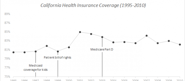
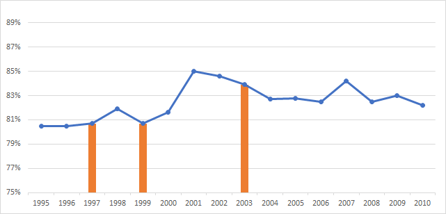
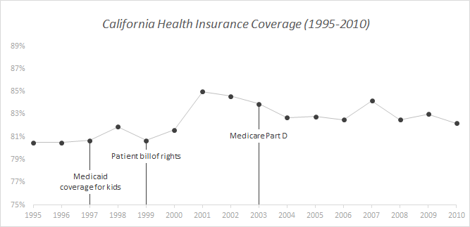
What?s in this article: A step-by-step guide I have laid out, for creating a time-series chart with events markers that change dynamically. While some of us use Python libraries, the vast majority of the world still uses Excel for good reasons, and hence the guide (or at least this first version) is for Excel. At the end of this tutorial, you will be able to produce something like this:

Showing change over time is a very common data visualization need for many analysts and researchers. Usually this is done by showing a line graph with X-axis representing time and Y-axis for the quantity of interest. Sometimes, we need to show particular events in addition to the time-series data, in order to highlight certain points. There are many ways to do this in Excel:
- The simplest but least flexible method is to just draw some lines and text boxes onto the line graph (not recommended).
- Another method is to use Y-error bars for some data points, which is a decent method but gets cumbersome as soon as your start making changes to data.
- The method shown here relies on creating two series on different axes ? one for actual quantity of interest and another for event markers. Once done, minimal changes are required for updates.
The completed version of this tutorial in Excel format is available here if you wish to practice on your own. So let?s get started.
Step 1: Get the data into shape
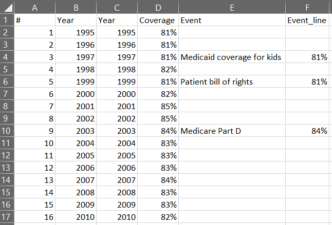
For this example, I used publicly available health insurance coverage data of California (available here) and identified some key events from the timeline given here. While I had to use some quick pivot table tricks to get the data into the required shape, those steps depend on your data source and are not discussed. Basically the data should have the following columns:
- Time series data for X-axis: In the figure below, this is the Year column but can be any time-scale (Yes there are two year columns, I will explain shortly).
- Data for quantity of interest: Here, this is the Coverage column, representing percent of population that has health insurance in the corresponding year.
- Events: This column contains names of event to be shown, against a specific year (Event column in figure below).
- Event marker length: This column contains the length of the event marker bar/line (Event_line column in figure below). In this example, I am setting this column equal to the Y-axis data point for the same event, and only for the data points where there is an event. But once you understand this, you can try many interesting variations. Important: where there is no event to be shown, both Event and Event_line are blank.
Why are there two Year columns? Because I wanted to explain a fairly common issue with how Excel treats dates and numbers differently. The first Year column (Column B) in the example above is simple a list of numbers I pasted from the source data. Excel does not recognize it as a date. The second column (Column C) is the actual Year column being used for the graph; it contains a formatted date that Excel recognizes on a date-time scale. To get the second column values from the first column, we need a simple formula. E.g. the formula in cell C2 is: = DATE (B2, 1, 1) which basically takes the number 1995 in cell B2 and converts into the date Jan 1st, 1995. The cell C2 is then formatted using a custom date format of Excel (yyyy) to show only the year part (see below).
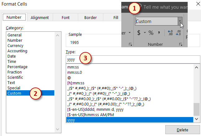
The date formatting steps are dependent on the scale you are using, but you can adapt the same method depending on whether you are using a month, day, or even hour, minute or second scale.
Why do this instead of using the numbers for X-axis? We could skip this, but then it will not work whenever the date/time sequence is uneven. With date-time recognized in Excel, it can deal with missing dates nicely.
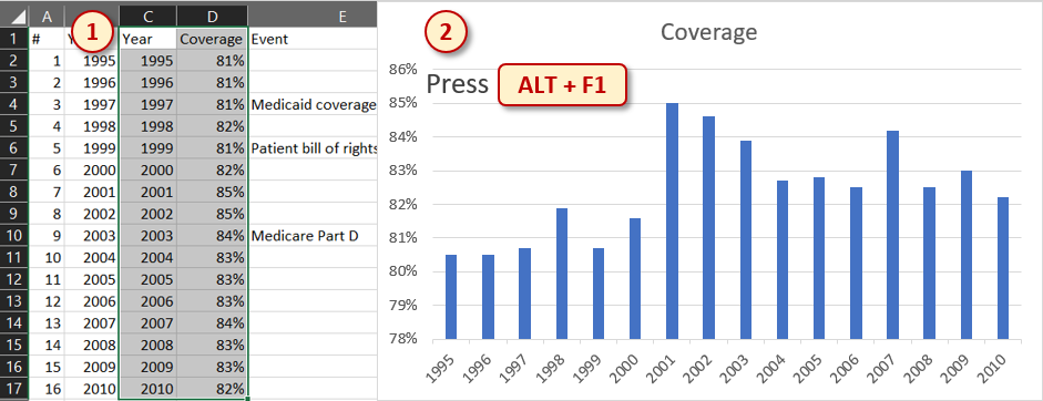
Step 2: Create a line chart
Select the two columns containing the time-series data and the quantity of interest (Columns C and D in figure below), and press Alt + F1. This is the quickest way to create a default chart using the selection.
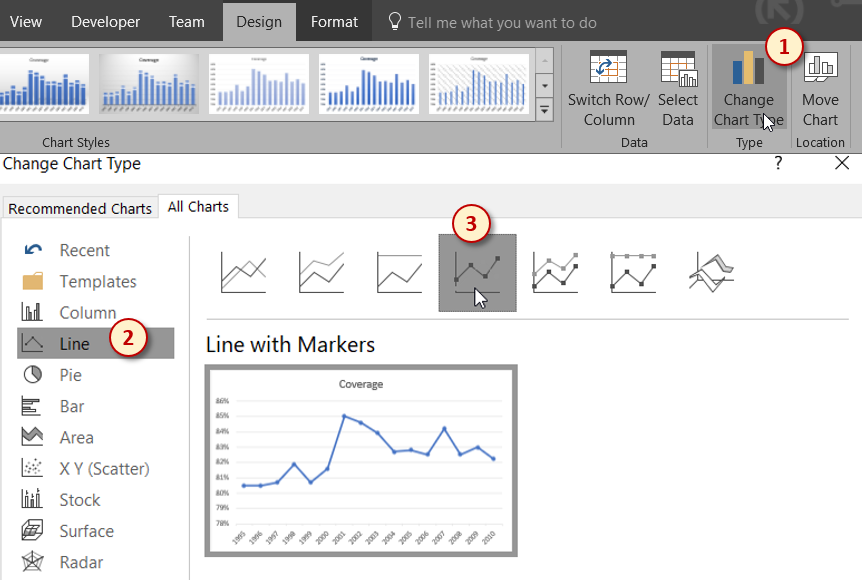
Next, change the chart type to Line and select the Line with Markers option (see below).
Now you should have a simple line chart with markers showing the change over time.
Step 3: Create event markers
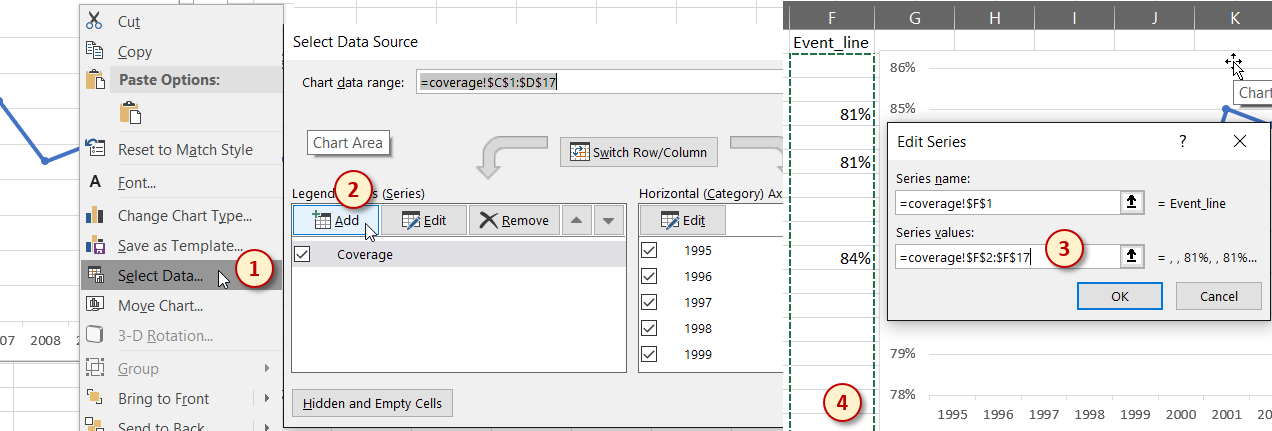
Now we need to add the event markers as another series to the chart. Remember that we need to set the values of event markers (Event_line column) same as the value of the Y-variable at the same year. I have done this simply by referring to the Y-values for the event years. E.g. cell F4 has the formula =D4. To add this Event_line column to the chart, right-click the chart and click ?Select Data??. In the dialogue box, click on the ?Add? button as shown below. Then in the next dialogue box, for the ?Series values? select all the values of the Event_line column (Column F) including the empty ones. Click OK and OK to finish adding series.
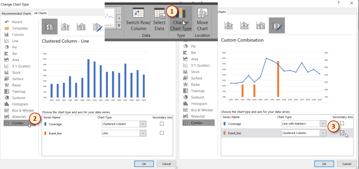
At this point, the event markers are added as another set of dots on top of the original Y-values and are hardly visible. But we want bars dropping from these points on the line graph down to the X-axis. For that, we need to convert this second series of data points to a cluster bar type. To do so, click on Change Chart Type option for the chart, select ?Combo? from the left column in the dialogue box, and then make sure that the original Y-values series (Coverage in this example) is set to ?Line with Markers? and the event markers series (named Event_line here) is set to ?Clustered Columns? and Secondary Axis is also selected for the latter.
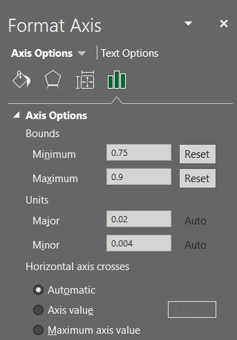
Now we are beginning to see light at the end of the tunnel. The bars however are now on a secondary axis. In order for the bars to exactly touch the dot markers on the line chart, both primary and secondary Y-axes need to be set exactly same. To do this, double click on the left Y-axis to open up the properties box and then set the Minimum and Maximum values of the axes as desired. In the figure below, I?ve set these to 0.75 (or 75%) and 0.90 (or 90%). Then repeat the same process for the right Y-axis.
Now, select the right sided Y-axis and press the Delete key to remove it. At this point, your chart should look something like this:
Step 4: Beautify (simplify)
Technically, the above chart is showing what we want to show, but now we shall apply some design principles to clean it up and improve the appearance significantly. This is what separates an amateurish attempt from a professional looking chart. Let?s do the following to make it awesome:
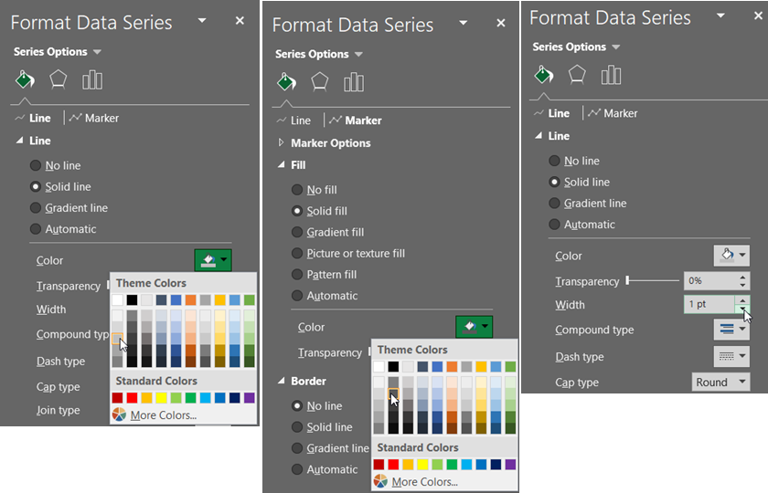
- Improve readability of line graph: Double click anywhere on the line to open its properties and change the color of line to very light gray and that of dot markers to a darker gray (but never full black). Also change the weight of the line to 1 pt. If you feel like it, increase the marker size to 6 pt.
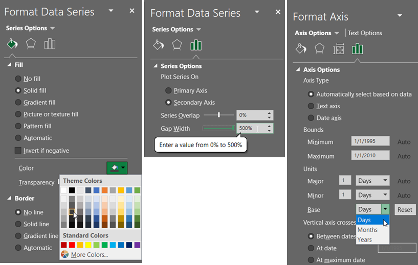
- Make the event bars thin and clear: Double click any of the bars to open their properties, and then set the border to ?No line? and change the Fill to a dark gray. Under the ?Series Options? tab in the same property box, move the ?Gap Width? slider to maximum value (500%). Now click on the X-axis to show its properties, and under the ?Axis Options?, change the ?Base? to Days. This squishes the bars even further to create the appearance of a thin line.
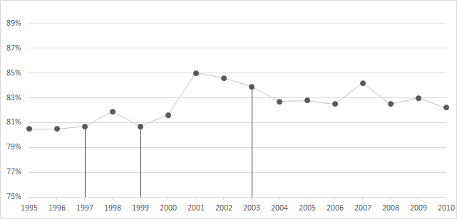
At this point, your chart should be close to this:
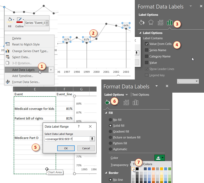
- Adding event labels: Right click on any of the bars and click ?Add Data Labels?. Now double click any of the data labels shown to open their properties box. Choose the ?Label Options? tab, deselect ?Value? and instead choose ?Value From Cells?. At this point you will see a small dialogue box asking for range of cells to pick values from. We need to click and drag to select the column containing the names of the events (Column E in this example). Then click OK to close this box. Now you should see the event names as data labels. They might be jumbled up and you can tweak their position either by choosing various label position options in the property box or manually adjusting them one by one. Finally, I like to give the labels a white fill so that any lines in the background don?t interfere with the text. You can also add a title to the chart now.
- Some more tweaking (optional): For both X and Y axes, I like to fade the text color to a lighter shade of gray but it depends on purpose of chart. In Edward Tufte?s spirit of reducing chart junk, I would also remove the horizontal grid lines by clicking them and pressing delete. However, this is also something that depends on the purpose of chart.
Congratulations! Now you have a refined, timeline chart with event labels nicely showing. I hope you found it useful. Please do leave feedback and comments.
Download the completed tutorial file here.
 California Health Insurance Coverage (Example of timeline chart with events)
