Often in Machine Learning we come across loss functions. For someone like me coming from a non CS background, it was difficult for me to explore the mathematical concepts behind the loss functions and implementing the same in my models. So here, I will try to explain in the simplest of terms what a loss function is and how it helps in optimising our models. I will consider classification examples only as it is easier to understand, but the concepts can be applied across all techniques.
Firstly, we need to understand that the basic objective of any classification model is to correctly classify as many points as possible. Albeit, sometimes misclassification happens (which is good considering we are not overfitting the model). Now, we need to measure how many points we are misclassifying. This helps us in two ways.
- Predict the accuracy of the model
- Optimising the cost function so that we are getting more value out of the correctly classified points than the misclassified ones
Hence, in the simplest terms, a loss function can be expressed as below.
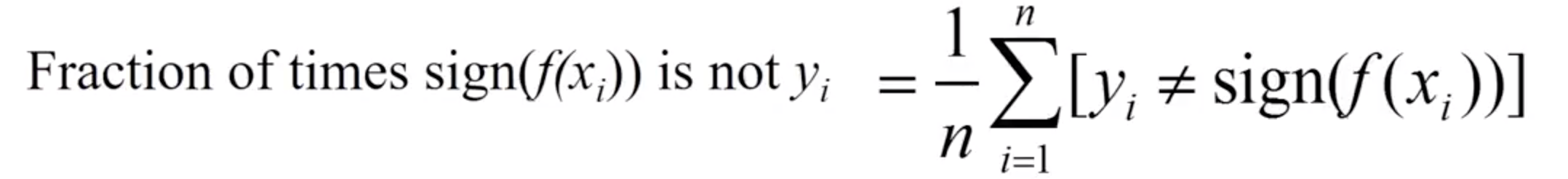 Fig 1 : Fraction of misclassified points
However, it is very difficult mathematically, to optimise the above problem. We need to come to some concrete mathematical equation to understand this fraction.
Let us now intuitively understand a decision boundary.
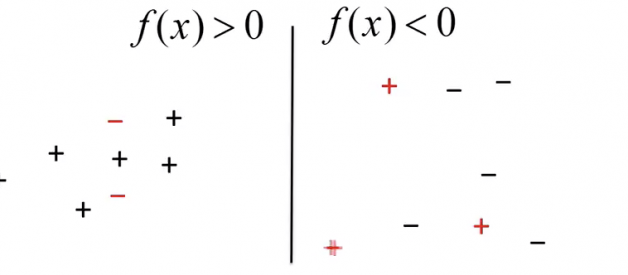
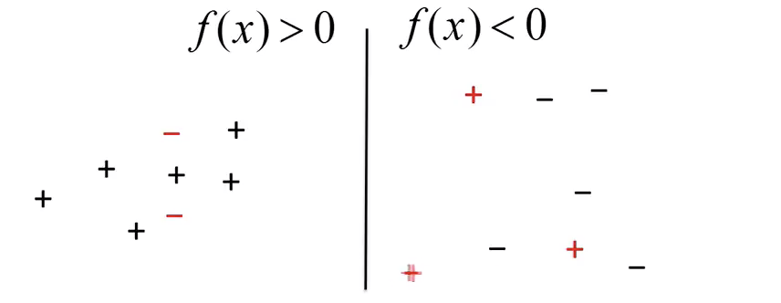 Fig 2: Decision boundary separating positive and negative points
The points on the left side are correctly classified as positive and those on the right side are classified as negative. Misclassified points are marked in RED.
Now, we can try bringing all our misclassified points on one side of the decision boundary. Let?s call this ?the ghetto?.
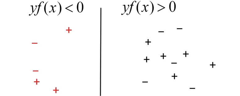 Fig 3: Misclassified points will always have a negative sign for yf(x)
From our basic linear algebra, we know yf(x) will always > 0 if sign of (?,?? ) doesn?t match, where ??? would represent the output of our model and ???? would represent the actual class label.
Now, if we plot the yf(x) against the loss function, we get the below graph.
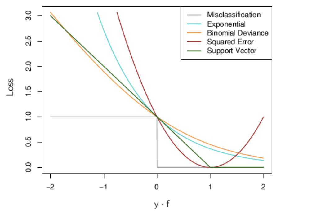 Fig 4: Plot of yf(x) with loss functions for various algorithms
Let us consider the misclassification graph for now in Fig 3. We can see that for yf(x) > 0, we are assigning ?0? loss. These points have been correctly classified, hence we do not want to contribute more to the total fraction (refer Fig 1). However, for points where yf(x) < 0, we are assigning a loss of ?1?, thus saying that these points have to pay more penalty for being misclassified, kind of like below.
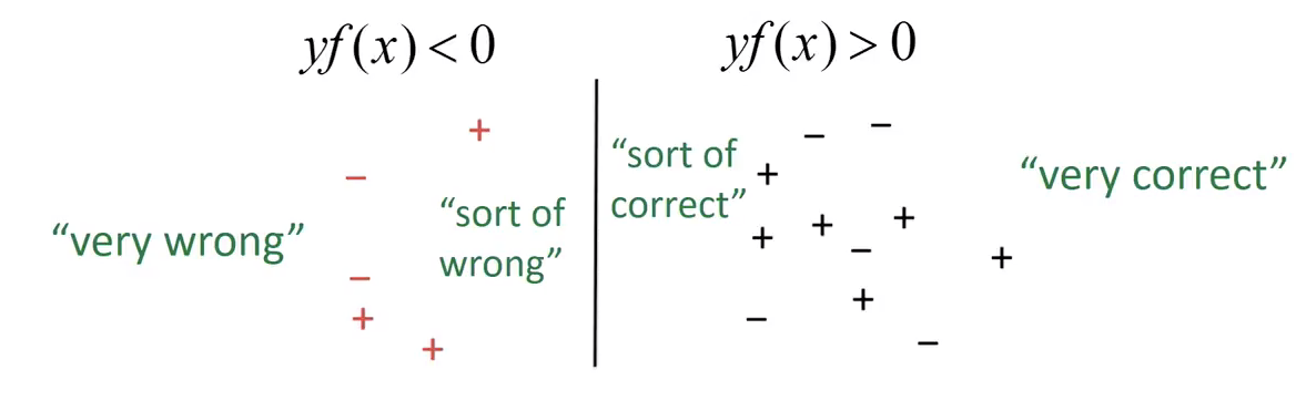 Fig 5: Loss function intuition
I hope, that now the intuition behind loss function and how it contributes to the overall mathematical cost of a model is clear.
Almost, all classification models are based on some kind of models. E.g. Logistic regression has logistic loss (Fig 4: exponential), SVM has hinge loss (Fig 4: Support Vector), etc.
From our SVM model, we know that hinge loss = [0, 1- yf(x)].
Looking at the graph for SVM in Fig 4, we can see that for yf(x) ? 1, hinge loss is ?0?. However, when yf(x) < 1, then hinge loss increases massively. As yf(x) increases with every misclassified point (very wrong points in Fig 5), the upper bound of hinge loss {1- yf(x)} also increases exponentially.
Hence, the points that are farther away from the decision margins have a greater loss value, thus penalising those points.
Conclusion: This is just a basic understanding of what loss functions are and how hinge loss works. I will be posting other articles with greater understanding of ?Hinge loss? shortly.
References :
Principles for Machine learning : https://www.youtube.com/watch?v=r-vYJqcFxBI
Princeton University : Lecture on optimisation and convexity : https://www.cs.princeton.edu/courses/archive/fall16/cos402/lectures/402-lec5.pdf

