Arrays are great for finding a piece of data, but costly to add or remove from. Hashes are easy to add or remove from, but costly to search. Both can show simple relationships, but become more difficult to read and traverse as these relationships, and the data associated with them, become more complex.
Arrays and hashes can be used to create data structures other than the classes provided to us in Ruby, like linked lists, trees, and graphs. In this blog post, we will be focusing on graphs. We will cover how to properly represent a graph in Ruby, and the two most common graph search algorithms: Breadth First Search and Depth First Search.
Simply put, a graph in computer science is a collection of connected items. We call these items nodes or vertices, and they are connected by edges. For instance, on Facebook, two users would each be represented by a vertex, and their friendship status would be represented by an edge. This connection allows for things like the ?People You May Know? feature, and seeing mutual friends with other users.
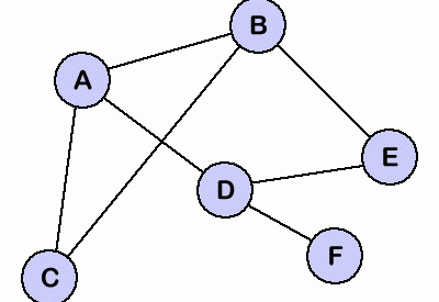
In the graph to the left, the vertices would be: A, B, C, D, E, and F.
The edges would be all of the lines you see connecting the vertices: A-B, A-C, A-D, B-C, B-E, D-E, D-F.
This is easy to see in a visual representation like this, but how can we represent this graph programmatically? The vertices can be stored in an array:
vertices = [‘A’, ‘B’, ‘C’, ‘D’, ‘E’]
This will work for now, however when we get into traversing graphs, we?ll see that we actually want to associate data with each node, and so an array of hashes (where each hash represent a node) is really the better option.
The edges can also be stored in an array, but this time, we will be using an array of arrays:
edges = [ [‘A’, ‘B’], [‘A’, ‘C’], [‘A’, ‘D’], [‘B’, ‘C’], [‘B’, ‘E’], [‘D’, ‘E’], [‘D’, ‘F’]]
Great! We now how a programmatic representation of our graph. We easily can return all of a node?s children, find out which nodes are vertices on this graph, and more. But we are definitely limited with what we can do here. As this graph scales, things like finding the shortest path between two nodes, and finding out if there is a path at all becomes much more complicated when the nodes aren?t adjacent.
Enter Breadth First Search and Depth First Search, the two most popular algorithms for traversing graphs. Wikipedia gives the below definition of graph traversal in computer science:
In computer science, graph traversal (also known as graph search) refers to the process of visiting (checking and/or updating) each vertex in a graph. Such traversals are classified by the order in which the vertices are visited.
Each of these represents a different approach to traversing, or visiting each vertex of, a graph.
Breadth First Search
BFS refers to the method in which you traverse a graph by visiting all children of a node before moving on to that child?s children. You can think in terms of levels. If the root node is Level 1, you visit all of Level 2, then all of Level 3, all of Level 4, and so on and so forth.
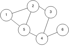
In the graph above, given a root node of 1, we would start at the node marked 1. Node 1 would be considered ?visited?, and we would then visit each of Node 1?s children, which would be Node 2 and Node 5. Now that we have visited all of Node 1?s children, Node 1 would be considered ?explored?, and Nodes 2 and 5 would be considered ?visited?. We then would visit Node 2?s unvisited children, which here would be Node 3. Node 2 is now explored, and Node 3 is visited.
Instead of going to Node 3?s children, we would go back to Node 5, and visit Node 5?s children. Again, we visit each ?level? before moving on, and 2 and 5 are of the same level here. So we visit Node 4, and mark Node 5 as having been explored.
Now we go back to Node 3 to visit its unvisited children, but it has none, so we mark it explored and go back to Node 4. We find Node 4?s only child, Node 6, mark it as visited and mark Node 4 as explored. We then see that Node 6 has no children, and there are no other unvisited vertices left to explore, so we mark Node 6 as explored and our algorithm completes.
If this feels confusing at first, that?s OK. Try to recreate the graph as vertices are marked explored, and you will see the pattern that we are moving in here.
Depth First Search
Whereas BFS goes level by level, DFS follows the path of one child as far as it can go, from root to finish, before going back and starting down the path of another child.
Using the same graph as above, and given a root node of 1, we would again start at the node marked 1, and visit each of Node 1?s children, Node 2 and Node 5. Instead of visiting Node 2?s unvisited children and then Node 5?s unvisited children, we visit Node 2?s unvisited children and continue to explore that path until we hit the end, before circling back to Node 5.
From Node 2 we visit Node 3 and mark Node 2 as explored. From Node 3 we visit Node 4 and mark Node 3 as explored, and from Node 4 we visit Node 6 and mark Node 4 as explored. We now see that we have nowhere to go from Node 6, so we mark it as explored, and circle back to Node 5. Because Node 5?s children have already been visited, we mark Node 5 as explored and our algorithm completes.
The Difference
You can see that changing the traversal approach results in nodes being explored at different points during the algorithm. This is a simple graph, so the differences are small, but below is the order in which vertices were marked explored using each algorithm:
BFS: 1, 2, 5, 3, 4, 6DFS: 1, 2, 3, 4, 6, 5
Notice that Node 5 goes from being the third vertex explored, to the last. These differences become greater as graphs become larger and more complex. Next week, we will tackle actually writing the code for the BFS and DFS algorithms using Ruby.

