Google Stock Predictions using an LSTM Neural Network

Deep Learning

Using a Vanilla LSTM for Stock Predictions

Time-series is a data format that is very tough to manage. Compared to cross-sectional data, a data format to which you can directly apply machine learning algorithms without preparing the data, predicting the future outcome of a Time-series invades the domain of Unsupervised Learning.

***DISCLAIMER: as exciting as it may look, this is a low-resolution simulation of a financial analysis model. Real-world models are much more complex, require Multi-variable data and are not limited to a single AI, but rather a collection of AI working together. Therefore, use this model for training on building Neural Networks Only: DO NOT ATTEMPT TO USE IT ON REAL TRADING, it will lack reliability due to its lack of complexity.

Full code available at my repository (including .cvs and notebook). If you only want to use the gist, click on this link.

Entire Procedure

In order to create a neural network capable of making predictions, I will use what is known as an LSTM (Long Short-Term Memory models). As mentioned before, we cannot use the same approach we have with supervised learning problems. Data needs to be prepared in a proper way so that the LSTM can process it:

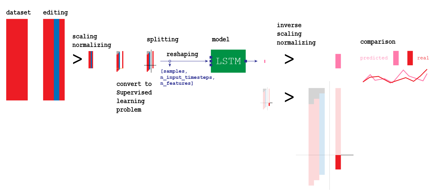Visualization of the entire model we are going to build

Steps in the process:

1. Importing Modules
2. Importing df
3. df preprocessing
4. df conversion to supervised problem
5. df splitting into X_train, y_train, X_test, y_test
6. Reshaping input into [samples, n_input_timesteps, n_features]
7. Create the LSTM model
8. Fit the model using X_train, y_train
9. Making an estimate for every single forward step
10. Invert preprocessing for the output
11. Invert preprocessing for the real values
12. Comparing predictions with estimations

tf_dataset_extractor

In order to speed up preprocessing, I will use my personal library called tf_dataset_extractor, available at this link. This library contains two classes for fast preprocessing. If you wish to know the details of every preprocessing step, you can simply look at the code inside.

import syssys.path.append(‘/content/drive/My Drive/Colab Notebooks/TensorFlow 2.0/modules’)import pandas as pdimport tf_dataset_extractor as e#import grapher_v1_1 as g#import LSTM_creator_v1_0 as lv = e.vl = e.l

I will begin by instantiating the two classes in tf_dataset_extractor:

• ?v? instantiates a class that contains cross-sectional data preprocessing algorithms
• ?l? instantiates a class that contains time series data preprocessing algorithms

GOOG Stock

#import datasetv.upload.online_csv(‘/content/drive/My Drive/Colab Notebooks/TensorFlow 2.0/csv/GOOG.csv’)e.K = v.upload.make_backup()

For your convenience, I have already saved the stock performance of 1 year of Google stock (GOOG) in a .csv file that you can download here. Because I use Google Colab, I will load it from my personal drive. You can download the .csv and import it from your own path.

Preprocessing

We will need two copies of the partitions we are going to create. The original copy will be normalized only, while the second one will be first normalized and then standardized. The reason for keeping both copies is that we will need to reconvert our output to its initial scale. I will explain the detailed procedure when we get to it.

Normalization only

#preprocessing with normalization onlyv.upload.retrieve_backup(e.K)#dropping extra columnse.X = e.X.drop([‘High’, ‘Low’, ‘Close’, ‘Adj Close’, ‘Volume’], axis=1)#preprocessingindex = e.X.pop(‘Date’)scaler, e.X = v.partition.scale(‘all_df’, scaler=’MinMaxScaler’, df=e.X, to_float=True, return_df=True)e.X = e.X.set_index(index)e.X = l.preprocessing.series_to_supervised(e.X, 3, 1)#X, yv.extract.labels([‘var1(t)’])#train, testX_train_, X_test_ = l.preprocessing.split(0.1, e.X)y_train_, y_test_ = l.preprocessing.split(0.1, e.y)e.X_ = e.X.copy()e.y_ = e.y.copy()print(X_train_.shape, X_test_.shape, y_train_.shape, y_test_.shape)

As we can see, all the variables we stored have an _ as a suffix to distinguish them from the rest of the other variables.

import matplotlib.pyplot as pltfig=plt.figure(figsize=(20, 10), dpi= 80)fig=plt.plot(e.y)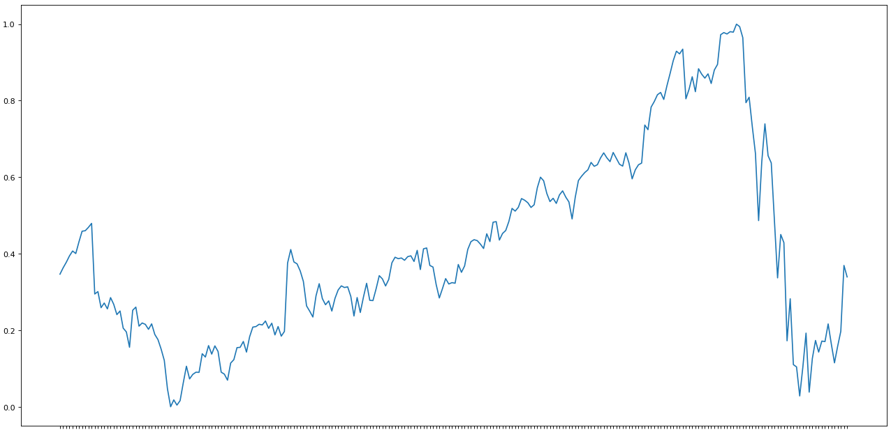

So far, our data has only been resized in the scale from 0 to 1.

Normalization + Standardization

#preprocessing with normalization and standardizationv.upload.retrieve_backup(e.K)#dropping extra columnse.X = e.X.drop([‘High’, ‘Low’, ‘Close’, ‘Adj Close’, ‘Volume’], axis=1)#preprocessingindex = e.X.pop(‘Date’)scaler, e.X = v.partition.scale(‘all_df’, scaler=’MinMaxScaler’, df=e.X, to_float=True, return_df=True)e.X = e.X.set_index(index)l.preprocessing.transform_to_stationary()e.X = l.preprocessing.series_to_supervised(e.X, 3, 1, drop_col=False)#X, yv.extract.labels([‘var1(t)’])#train, testX_train, X_test = l.preprocessing.split(0.1, e.X)y_train, y_test = l.preprocessing.split(0.1, e.y) #sembra non servire a nullaprint(X_train.shape, X_test.shape, y_train.shape, y_test.shape)

All the variables above have no _ as a suffix. We do not actually need to conserve all these copies. In reality, much of this code is not really necessary, but it will be easier for me to explain. Know that we will keep a normalized copy (defined with _ at the end of each variable) and a normalized + standardized copy of our entire df.

import matplotlib.pyplot as pltfig=plt.figure(figsize=(20, 10), dpi= 80)fig=plt.plot(e.y_)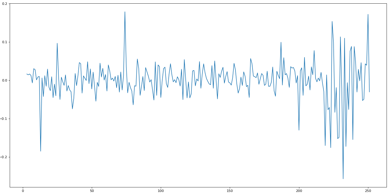

This is how a normalized + standardized preprocessing looks like. We will feed this data to the LSTM, and it will make predictions.

Input and Output

During preprocessing, we isolated the datasets e.y and e.X. If we look at the two datasets before splitting, essentially this is what we end with:

• Input

e.X.head()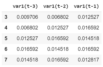import matplotlib.pyplot as pltfig=plt.figure(figsize=(20, 10), dpi= 80)fig=plt.plot(e.X)

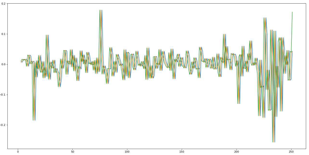
We just took the stock dataset at time 0, and we shifted three times, storing each shift in a different column, resulting in the graph above. This is called lag. The LSTM will look at three steps backward to make a one-step future prediction.

• Output

e.y.head()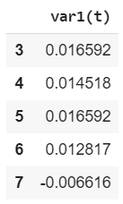

We will be using the labels to train the LSTM. In this case, we want out LSTM to look at only one step in the future, therefore only one column.

Splitting

As you can see in written in the code above will be splitting our dataset in X_train, y_train, X_test, y_test. We will use the training sets to train our AI, X_test to make predictions, and finally, y_test to make a comparison between estimations and real data.

Preparing the input for the LSTM

As input, we will use our column var1(t). Because its original shape is (225, 3), we will need to reshape it in a form the LSTM can comprehend: [samples, n_input_timesteps, n_features].

#reshape [samples, n_input_timesteps, n_features]X_train = X_train.reshape((225, 3, 1))y_train = y_train.reshape((225, 1, 1))print(X_train.shape, y_train.shape)#every individual sample has dimensions [1, 3, 1]

Every individual sample, for example, the first line:

X_train[0]array([[0.00970626], [0.00680232], [0.01252675]])

Will have dimensions (1, 3, 1).

Vanilla LSTM

We can finally create the model for our neural network. The LSTM I am going to use is called a Vanilla LSTM, is a simple form of neural network for Univariate Time-series predictions, it only contains a dense layer:

#LSTM%tensorflow_version 2.ximport tensorflow as tffrom tensorflow.keras import Sequentialfrom tensorflow.keras import layersfrom tensorflow.keras.layers import Densefrom tensorflow.keras.layers import LSTMmodel = Sequential()model.add(LSTM(50, batch_input_shape=(1, 3, 1), stateful=True))model.add(Dense(1))model.compile(loss=?mean_squared_error?, optimizer=?adam?)model.fit(X_train, y_train, epochs=3000, batch_size=1, verbose=2, shuffle=False)model.reset_states()X_test = X_test.reshape(24, 3, 1)y_test = y_test.reshape(24, 1, 1)print(X_test.shape, y_test.shape)…Epoch 2998/3000 225/225 – 0s – loss: 1.7274e-04 Epoch 2999/3000 225/225 – 0s – loss: 2.9163e-04 Epoch 3000/3000 225/225 – 0s – loss: 2.8836e-04 (24, 3, 1) (24, 1, 1)

Prediction

We can store our predictions in a list called yhat:

#make a one-step forecastyhat = model.predict(X_test, verbose=2, batch_size=1) #without batch_size the model only accepts one input at a timeyhat24/24 – 0s [[ 0.0721423 ] [-0.13979942] [ 0.02534528] [-0.15360811] [ 0.04295617] [ 0.14269553] [ 0.06470203] [ 0.02760611] [ 0.03455507] [-0.13316691] [ 0.03844658] [-0.00989904] [ 0.08717629] [ 0.00703726] [-0.05191287] [ 0.00792047] [-0.0025476 ] [ 0.01022832] [ 0.06648263] [ 0.05616217] [ 0.03048991] [-0.02833473] [ 0.00622515] [-0.0042644 ]]

Unfortunately, as mentioned before, our predictions will come out with the same scale of the input, which has been normalized and then scaled. We will have to invert these processes to have a data scale we can actually compare.

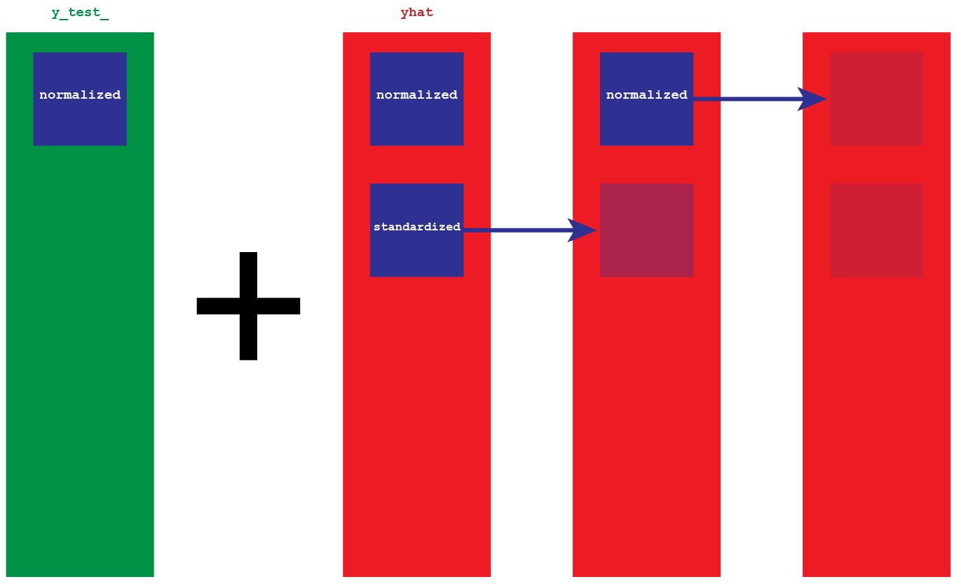
In order to invert the data, we will need the original copy of y_test_ and our predictions. y_test_ it is the real version of the data, therefore the scale we want to obtain (for ex. 1300, right now its equivalent number is .0009). Because the predictions yhat have been normalized and then stationarized, they are nothing but a collection of gaps. We will add those gaps to the normalized version of y_test_.

#invert preprocessing on predicted data#remove stationaryy_test = y_test.reshape(24, 1)var1 = y_test_ #original valuesvar2 = yhat #gapsvar3 = list() ##var1 = var1.values#var2 = var2.valuesvar3.append(var1[0])for i in range(0, len(var2)): values = var1[i] + var2[i] var3.append(values) var3

At this point, we still have our normalized version of the predictions. We invert the preprocessing, and we have them on a scale of thousands.

#inverse scalingpredicted = scaler.inverse_transform(var3)predictedarray([[1350.19995824], [1384.98480799], [1209.65298139], [1217.52072549], [1185.93480519], [1270.41216402], [1194.80344785], [1210.19733755], [1109.31081349], [1109.77145847], [ 992.30088891], [1111.58781353], [1130.94699481], [1103.35372615], [1107.16316306], [1101.43918236], [1115.61908397], [1124.44163555], [1129.97183253], [1179.35603071], [1149.07968629], [1112.96137088], [1105.35280738], [1141.00156137], [1218.94379394]])

Expectations

The labeled data that shows what really happened has only been normalized (that is why it has _ as a suffix). We will just need to bring it back to its normal scale by using the scaler we have been saving from the beginning.

#invert preprocessing on expected data#inverse scalingexpected = scaler.inverse_transform(y_test_)expectedarray([[1350.2 ], [1277.06 ], [1205.3 ], [1260. ], [1249.7 ], [1126. ], [1179. ], [1096. ], [1093.11 ], [1056.51 ], [1093.05 ], [1135.72 ], [1061.32 ], [1103.77 ], [1126.47 ], [1111.8 ], [1125.67 ], [1125.04 ], [1147.3 ], [1122. ], [1098.26 ], [1119.015], [1138. ], [1221. ], [1206.5 ]], dtype=float32)

Comparison

We are ready to compare the predicted with the expected values to see how close they are:

for i in range(len(y_test_)): print(‘iteration=%d, Predicted=%f, Expected=%f’ % (i+1, predicted[i], expected[i]))iteration=1, Predicted=1350.199958, Expected=1350.199951 iteration=2, Predicted=1384.984808, Expected=1277.060059 iteration=3, Predicted=1209.652981, Expected=1205.300049 iteration=4, Predicted=1217.520725, Expected=1260.000000 iteration=5, Predicted=1185.934805, Expected=1249.699951 iteration=6, Predicted=1270.412164, Expected=1126.000000 iteration=7, Predicted=1194.803448, Expected=1179.000000 iteration=8, Predicted=1210.197338, Expected=1096.000000 iteration=9, Predicted=1109.310813, Expected=1093.109985 iteration=10, Predicted=1109.771458, Expected=1056.510010 iteration=11, Predicted=992.300889, Expected=1093.050049 iteration=12, Predicted=1111.587814, Expected=1135.719971 iteration=13, Predicted=1130.946995, Expected=1061.319946 iteration=14, Predicted=1103.353726, Expected=1103.770020 iteration=15, Predicted=1107.163163, Expected=1126.469971 iteration=16, Predicted=1101.439182, Expected=1111.800049 iteration=17, Predicted=1115.619084, Expected=1125.670044 iteration=18, Predicted=1124.441636, Expected=1125.040039 iteration=19, Predicted=1129.971833, Expected=1147.300049 iteration=20, Predicted=1179.356031, Expected=1122.000000 iteration=21, Predicted=1149.079686, Expected=1098.260010 iteration=22, Predicted=1112.961371, Expected=1119.015015 iteration=23, Predicted=1105.352807, Expected=1138.000000 iteration=24, Predicted=1141.001561, Expected=1221.000000 iteration=25, Predicted=1218.943794, Expected=1206.500000

Graphing

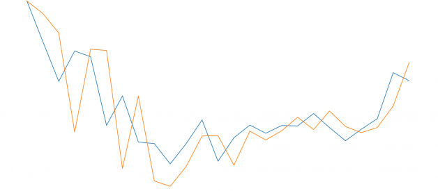
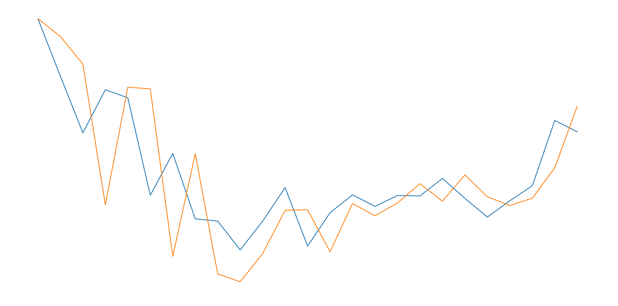
import matplotlib.pyplot as pltfig=plt.figure(figsize=(20, 10), dpi=80)fig=plt.plot(expected)fig=plt.plot(predicted)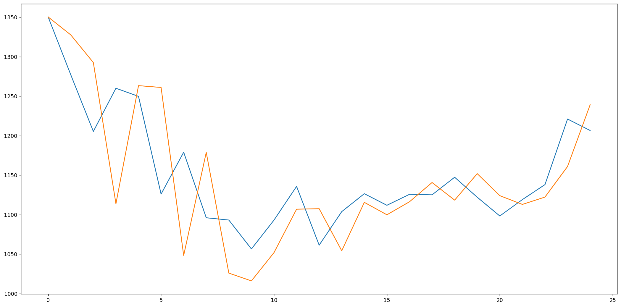

Evaluating Performance

As we can see, the model is not too accurate. However, in the stock market, we cannot simply make predictions based on a single variable, it would not be realistic; that is why we need more complex models for estimations.

# report performancefrom math import *from sklearn.metrics import mean_squared_errorrmse = sqrt(mean_squared_error(expected, predicted))print(?Test RMSE: %.3f? % rmse)Test RMSE: 58.232