 Depth-first search graph traversal
For better or for worse, there?s always more than one way to do something. Luckily for us, in the world of software and computer science, this is generally a Very Good Thing?.
And why is it good? Well, for one, I?m a big fan of options and having many of them to choose from. But really, it all comes down to different types of problems ? some of which can seem similar to things we?ve seen before ? and the various solutions that fit best to solve them. This is certainly the case for the seemingly simplest of problems: take sorting, for example. As we learned early on in this series, there so many different methods of doing something as basic as sorting a series of numbers and putting them in order. In fact, the multiplicity of options is often exactly what makes a task that ought to be ?basic? seem far more complicated.
Here?s the thing, though: if we can get manage to climb over the hump of over-complication and somehow make it over to the other side, then we can start to see that all of these various solutions arose from a need to solve similar, but ever-so-slightly different problems. That was certainly the case with the origins of many of the sorting algorithms we know (and hopefully love!), and it?s the case with graph traversal algorithms, too. Last week, we learned about one approach to the problem of walking through a graph: breadth-first search. Today, we?ll flip this approach on its head, and look at a solution that is similar, and yet also the inverse of BFS.
So, without further ado: let?s dive right into the deep end, shall we?
A primer, before going deep
A helpful first step in knowing how any algorithm works and what it does is by knowing what the algorithm does not do. In other words, when we?re learning something new, it can be useful to compare the new thing that we?re learning to the things that we already know well and feel fairly comfortable with.
This is particularly the case when we start getting into more complex algorithms, like graph traversal algorithms. So, let?s start with a definition, and then see how depth-first search compares to the other graph traversal algorithm that we are already familiar with: breadth-first search.
 Depth-first search: a definition
The depth-first search algorithm allows us to determine whether two nodes, node x and node y, have a path between them. The DFS algorithm does this by looking at all of the children of the starting node, node x, until it reaches node y. It does this by recursively taking the same steps, again and again, in order to determine if such a path between two nodes even exists.
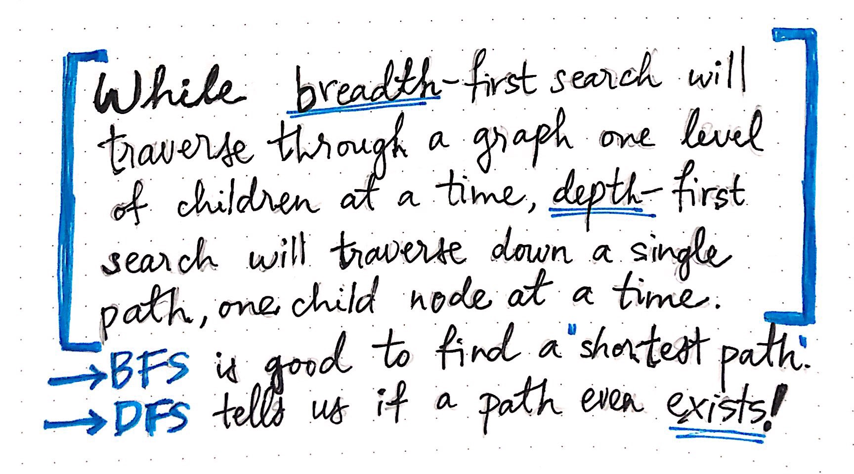
Now, if we contrast DFS to what we know about BFS, or breadth-first search, we?ll start to see that, while these two algorithms might seem similar, they are fundamentally doing two very distinct things. The striking difference between the two algorithms is the way they approach the problem of walking or traversing through the graph. As we discovered last week, the BFS algorithm will traverse through a graph one level at a time, visiting all the children of any given vertex ? the neighboring nodes that are equidistant in how far away from the ?parent? node in the graph.
 Comparing DFS to BFS graph traversal
However, depth-first search takes a different approach: it traverse down one single path in a graph, until it can?t traverse any further, checking one child node at a time.
The depth-first algorithm sticks with one path, following that path down a graph structure until it ends. The breadth-first search approach, however, evaluates all the possible paths from a given node equally, checking all potential vertices from one node together, and comparing them simultaneously.
Like architecture and biology, in this case, the old adage rings true: form really does follow function. That is to say, the way that both of these algorithms are designed help give us clues as to what their strengths are! Breadth-first search is crafted to help us determine one (of sometimes many) shortest path between two nodes in the graph. On the other hand, depth-first search is optimized not to tell us if a path is the shortest or not, but rather to tell us if the path even exists!
And, as we can probably imagine, different situations, problems, and graphs will lead us to choose one of these algorithms over another. But, we?ll come back to this later on. For now, let?s just focus on getting to know depth-first search a little better.
Depth-first search is a particularly interesting algorithm because it?s likely that we?ve all used some variation of it at some point in our lives, whether we realized it or not. The easiest way to reason about depth-first search in a graph is to simplify it into a much easier problem.
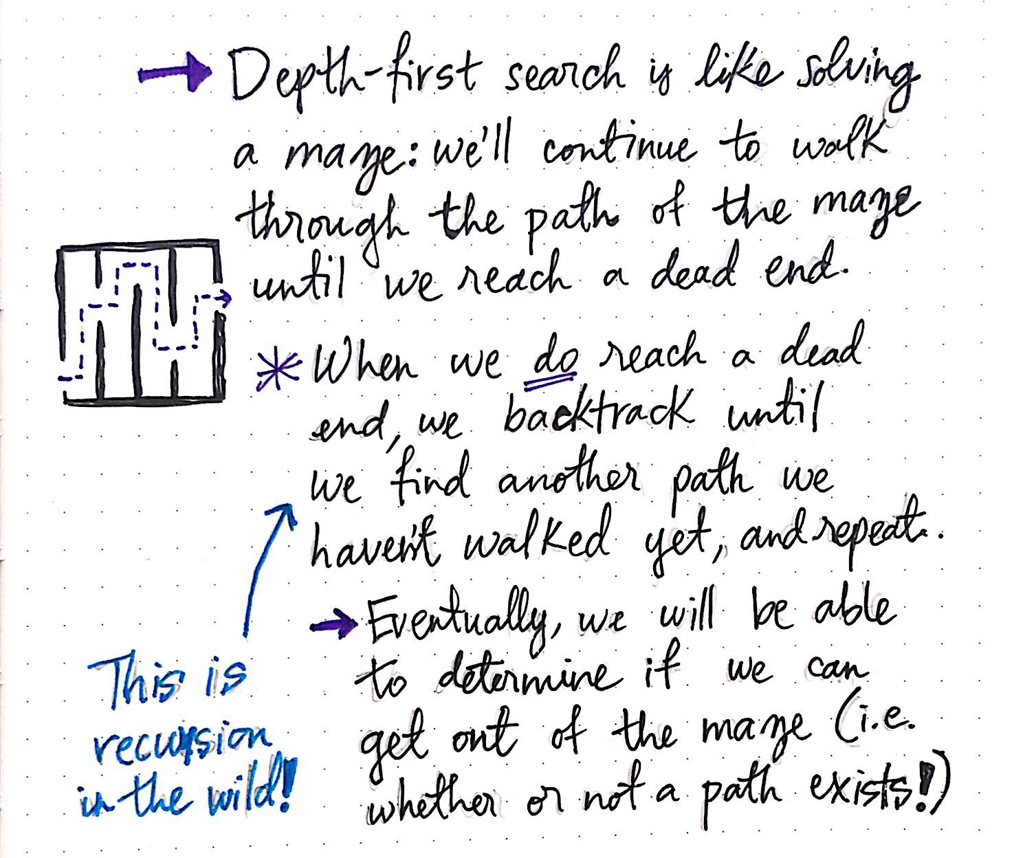 Depth-first search: solving a maze
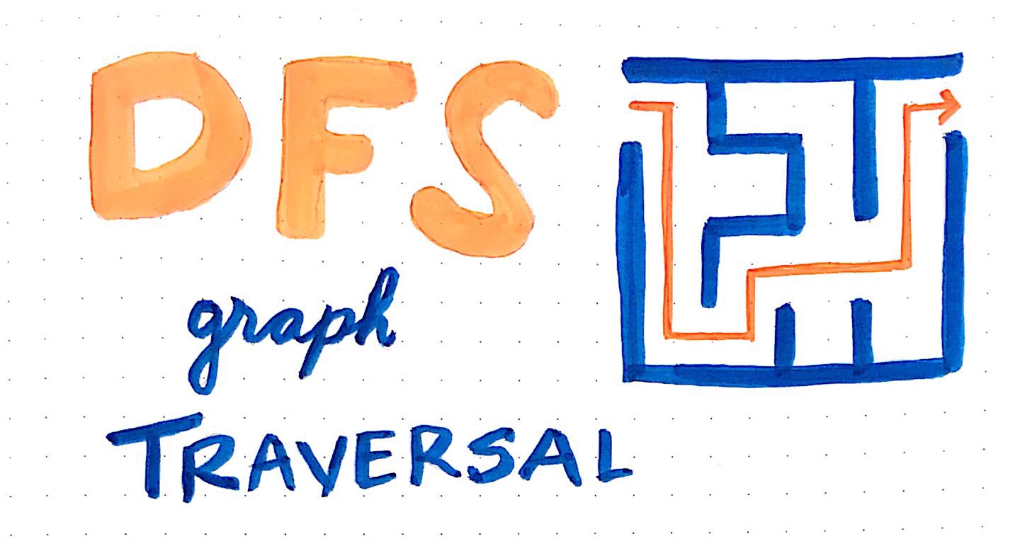
The DFS algorithm is much like solving a maze. If you?ve ever been to a real-life maze or found yourself solving one on paper, then you know that the trick to solving a maze centers around following a path until you can?t follow it anymore, and then backtracking and retracing your steps until you find another possible path to follow.
At its core, that?s all that the depth-first search algorithm really is: a method of getting out of a maze! And, if we envision every graph as a maze, then we can use DFS to help us ?solve? and traverse through it.
Using this metaphor, when we employ DFS, all we?re really doing is continuing to walk through the path of a graph until we reach a dead end. If and when we reach a dead end, we backtrack until we find another path that we haven?t yet traversed through or walked down, and repeat the process. Eventually, we?ll be able to determine whether or not we can get out of the maze ? that is to say, whether or not a path between the starting node and the ending node exists.
One interesting thing to note before we start putting all this DFS theory into practice: the process of backtracking at a dead end and then repeating the walk down one single path of a graph is actually just recursion! We?re taking the same action again and again and, in programmatic terms, this would end up being a recursive function call, or a function that calls itself until it hits some sort of base case. As we?ll see in a moment, recursion plays a big part in how DFS actually runs.
Depth-first, in action
Exactly like what we saw in last week?s exploration of BFS, we can start our traversal of a graph with DFS in a similar fashion ? wherever we want!
When it comes to both breadth-first search and depth-first search, there are only two major points to keep in mind when initiating a graph traversal: first, we can choose any arbitrary node to start our traversal with, since there is no concept of a ?root? nodes the way that there are in tree structures. And second, whatever we do, we want to ensure that we don?t repeat any nodes; that is to say, once we ?visit? a node, we don?t want to visit it again. Similar to what we did with the breadth-first search algorithm, we?ll mark every vertex we visit as ?visited? in order to ensure that we don?t repeat nodes in our traversal unnecessarily.
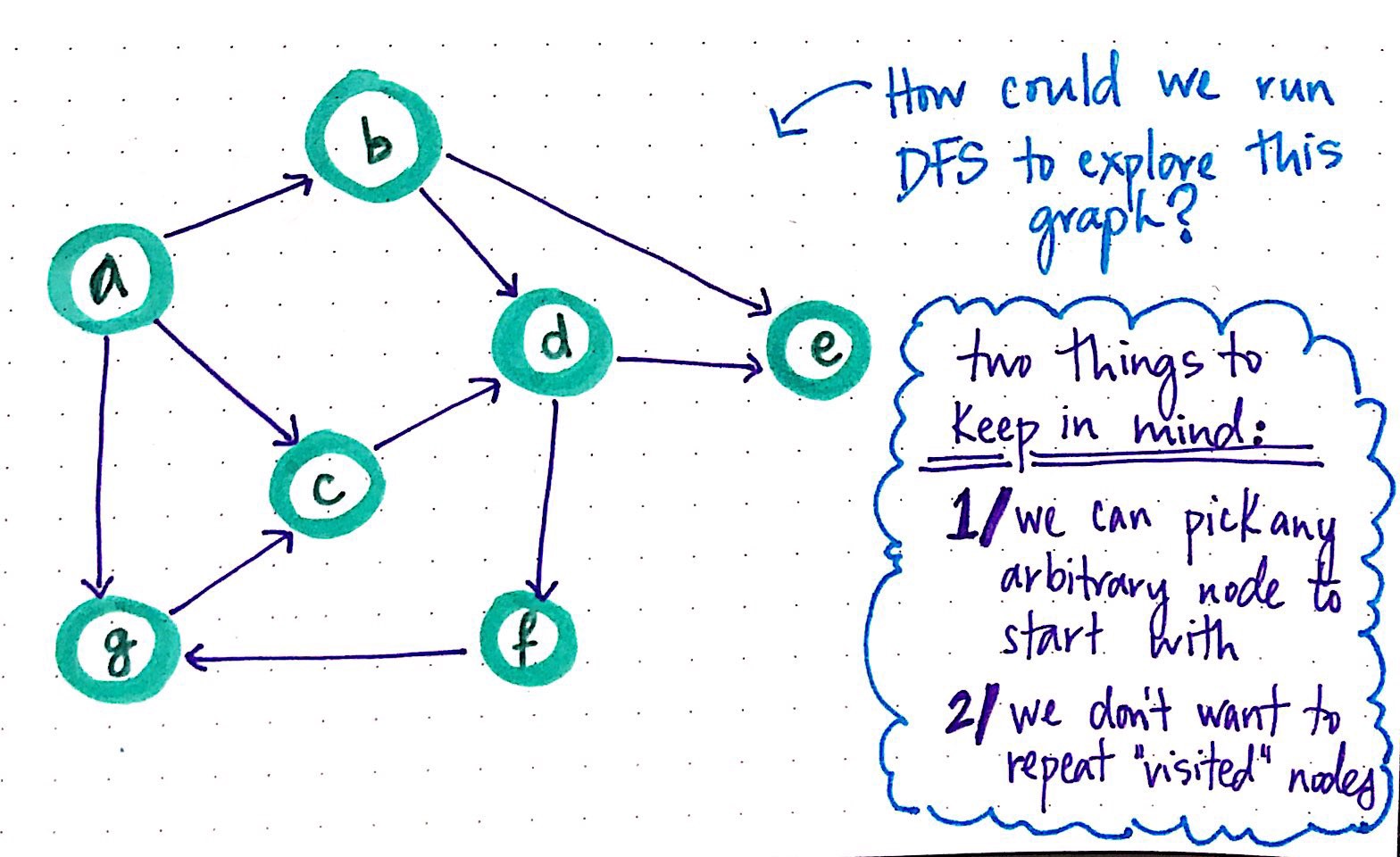 How could we run DFS to explore a directed graph?
So, let?s try to run a DFS algorithm on the directed graph above, which has seven nodes that we?ll end up needing to check, or ?visit? in the course of our graph traversal.
We can arbitrarily choose any node to start with, let?s choose node a as our starting ?parent? node. Since we know that depth-first search is all about finding out whether a path exists or not between two nodes, we?ll want to be sure that we can keep track of where we came from as we walk through our graph ? in other words, we?ll need to keep some kind of trail of ?breadcrumbs? as we traverse.
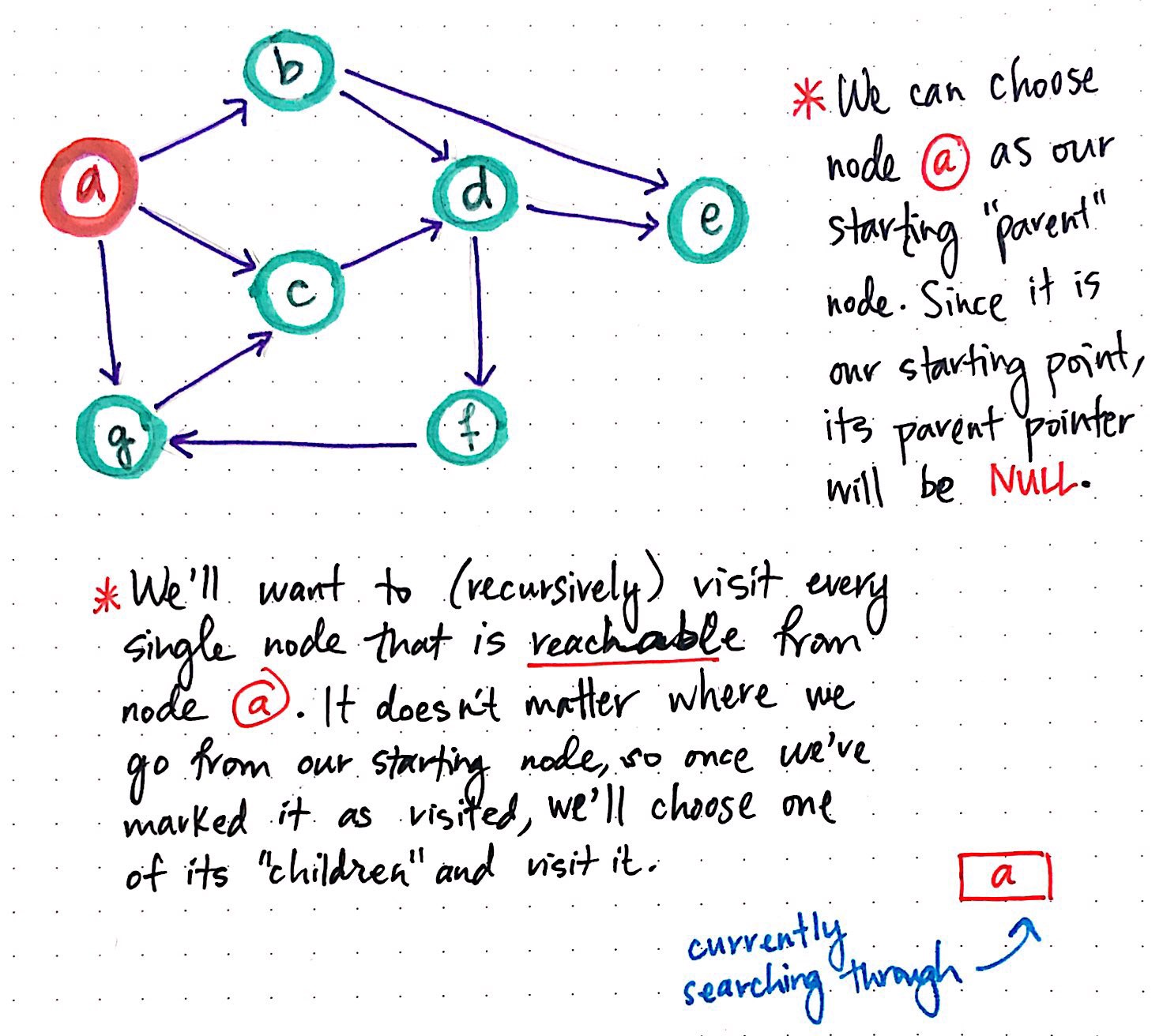 DFS, part 1
For every node that we visit, we?ll keep track of where we came from and use that to both backtrack when we need to, and also as an easy way to keep track of the path that we?re constructing through the graph. When we choose node a as our ?parent? node, we?ll set a parent pointer reference, just like we did with our BFS algorithm. Since the ?parent? vertex is the first one we?re visiting in this algorithm, it doesn?t have a ?parent? pointer, since we?re not coming from anywhere!
So, we?ll set node a’s parent pointer to NULL, and mark node a as ?visited?. A simple way to keep track of which node we?re currently searching through is by employing a stack data structure. The moment that we check node a, we can push it right on top of our stack. Since our stack is empty to start with, node a is the only element that?s actually in our stack. We?ll mark it as ?visited?.
Next, we?ll want to (recursively) visit every single node that is reachable from node a. Just as it doesn?t matter which node we start with, it doesn?t really matter which neighboring vertex we visit next ? just as long as the vertex is reachable, and is one of the neighbors of a. For example, we could arbitrarily choose to visit node c next.
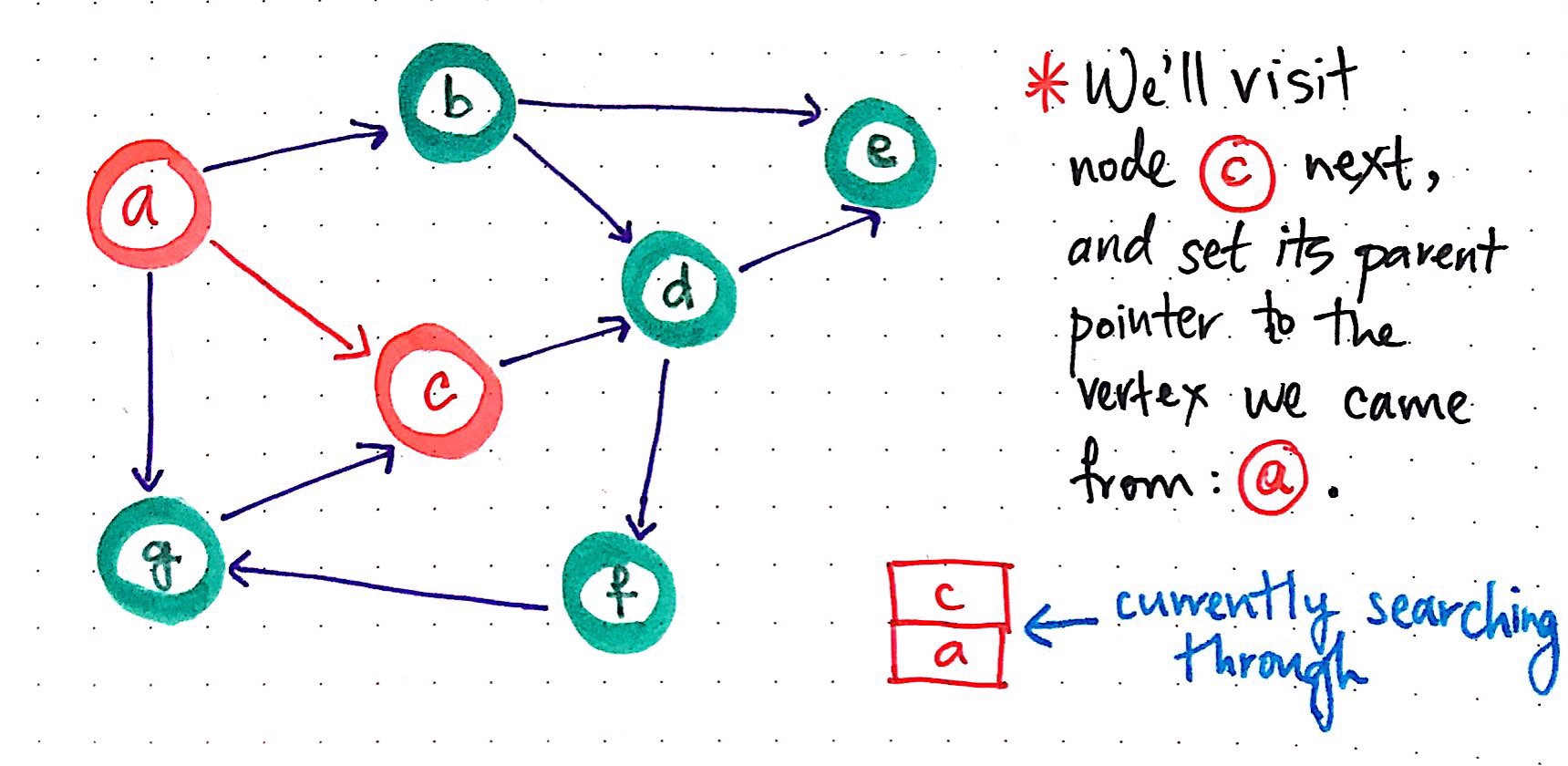 DFS, part 2
We?d push it onto the stack, which now contains two elements ? a reference to node a as well as a reference to node c?and we?ll visit the node that is currently on top of the stack. In the process, we?ll set its parent pointer to the vertex that we just came from: node a.
 DFS, part 3
Now that we?ve visited node c, there?s only one thing left to do: lather, rinse, and repeat! Okay, okay ? you can skip the first two. Really all we need to do here is just repeat the process (suds optional, obviously).
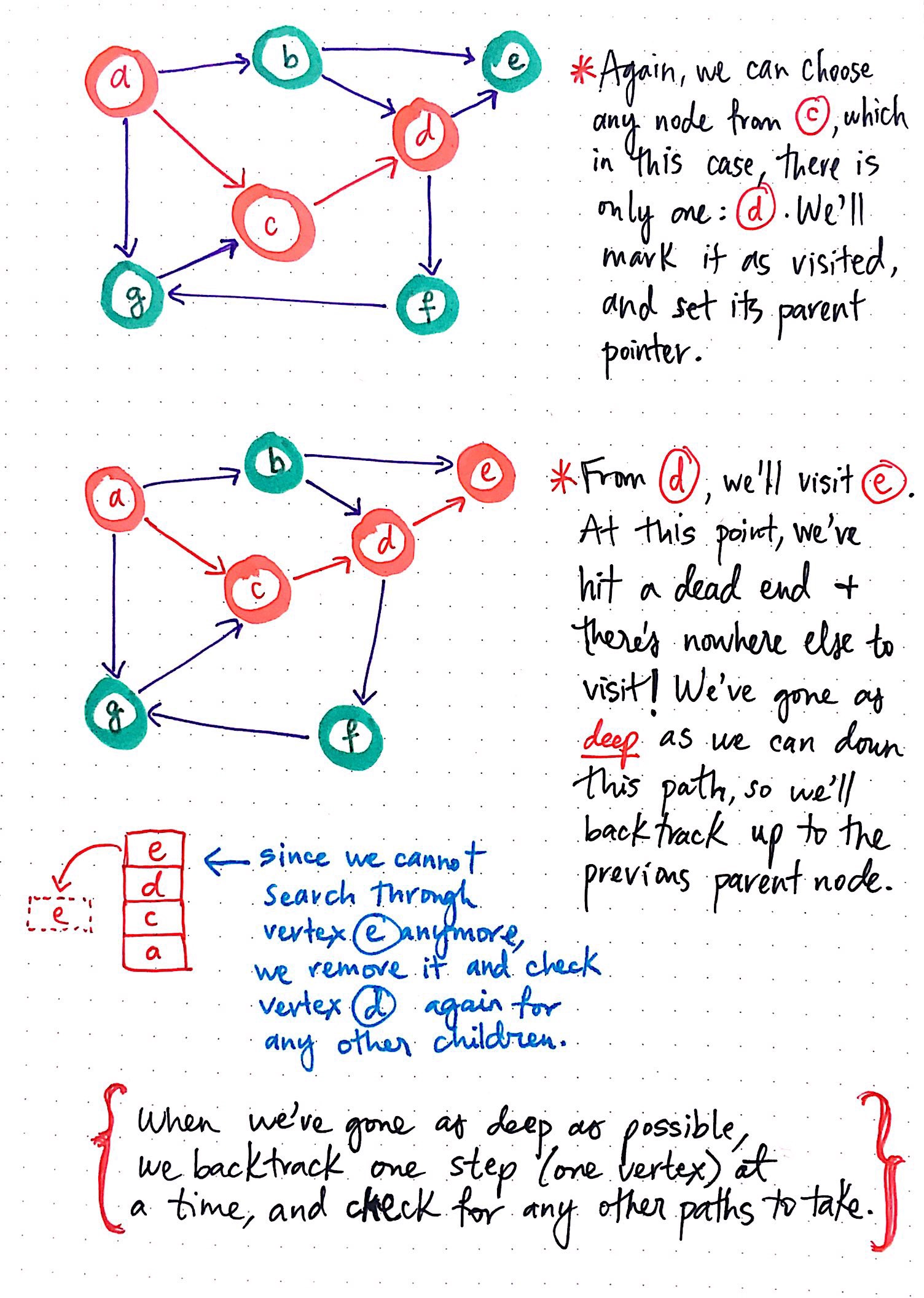
For example, since we can choose any node that is reachable from node c, we could choose node d as the next node we visit. We?ll add it to the top of the stack, mark it as ?visited?, and set its parent pointer.
From node d, we?ll visit node e: add it to the stack, mark as ?visited?, and finally, set its parent pointer to the node we just came from: node d.
But now we have a problem: we can?t repeat this process because there?s simply nowhere to go from node e!
We?ve gone as deep as we can down this particular path from the node that we started with, and we?ve hit a dead end; that is to say, we?ve reached a node with no reachable vertices!
Given our conundrum, let?s pause for a moment and take a look at our stack of ?visited? nodes, which has the following nodes on it: e, d, c, and a, in that order, from the top of the stack to the bottom. Since there is nowhere to go from node e, we effectively have no other node to visit, which means that we have no other node to add to the top of the stack. At least, given where we currently are, at node e. But, node d, the second element in the stack might have somewhere to go, right?
And this is exactly where the backtracking and the idea of ?breadcrumbs? comes into play ? not to mention recursion! When we?ve gone as deep as possible down the graph, we can backtrack one step (one vertex) at a time, and check to see if there are any other paths that we could possibly take.
So, since we can?t search through any paths from vertex e (since none exist), we?ll pop vertex e off of the top of the stack once we?re finished with it. This leaves node d at the top of the stack, so we?ll repeat the same process again ? that is to say, we?ll check to see if any of node d’s neighbors can be visited and if there is a path down the graph from that node.
 DFS, part 4
Once we backtrack from node e to d, we?ll notice that there?s only one direction for us to go; there is only one node to check, which is node f. We?ll add it to the top of the stack, mark it as visited, and check to see if it has any children that we an visit.
We?ll notice that, after we backtracked and changed which node we were checking, looking at, or ?visiting?, the top of the stack changed. We popped off some nodes, and added on others, but the main parent node remained the same. We repeated the same steps again and again, with each node that was added to the top of the stack ? and those steps were the same things we checked for the parent node, vertex a, when we added it to the stack when we first started out! This is recursion coming into play.
 DFS, part 5
From node f, we have no choice but to visit g, which is the only accessible node ? the only one that is available for us to visit. So, we?ll add g to the top of our stack, visit it, and check to see where we can go from there.
As it turns out, from node g, there is only one place for us to go: node c. However, since we were smart enough to keep track of the nodes that we visited, we already know that c has been visited and is part of this path; we don?t want to visit it again! So, we?ve come to another dead end, which means that we can backtrack. We?ll pop off node g from the stack, check to see if the next node has any other children we can traverse through. As it turns out, node f doesn?t have any child nodes that we haven?t already visited, nor do nodes d and c; so, we?ll pop all of them off from the top of the stack.
Eventually, we?ll find that we?ve backtracked our way all the way to our original ?parent? node, node a. So, we?ll repeat the process again: we?ll check to see which of its children we can visit, which we haven?t already visited before. Since we?ve already visited nodes c and g, the last remaining option is to visit b.
Again, we?ll do what we?ve done with every single node thus far: add node b to the top of the stack, mark it as ?visited?, and check to see if it has any children that we can traverse through that haven?t been visited yet. However, node b’s children are e and d, and we?ve visited both already, which means that we?ve actually visited all of the nodes in this graph! In other words, our depth-first graph traversal is officially complete for this structure.
We?ll notice that, with each node that we pushed and later popped off the stack, we repeated the same steps from within our depth-first search algorithm. Indeed, what we were really doing was recursively visiting nodes. Effectively, every time that we reached a new node, we took these steps:
- We added the node to the top of the ?visited? vertices stack.
- We marked it as ?visited?.
- We checked to see if it had any children ? and if it did, we ensured that they had not been visited already, and then visited it. If not, we popped it off the stack.
With every new node added to the stack, we repeated these steps from within the context of the previous node (or previous function call) on the stack. In other words, we recursively visited each node down the path, until we reached a dead end.
As it turns out, this recursive repetition of visiting vertices is the main characteristic of most implementations of the depth-first search algorithm!
Real-life recursion and runtime
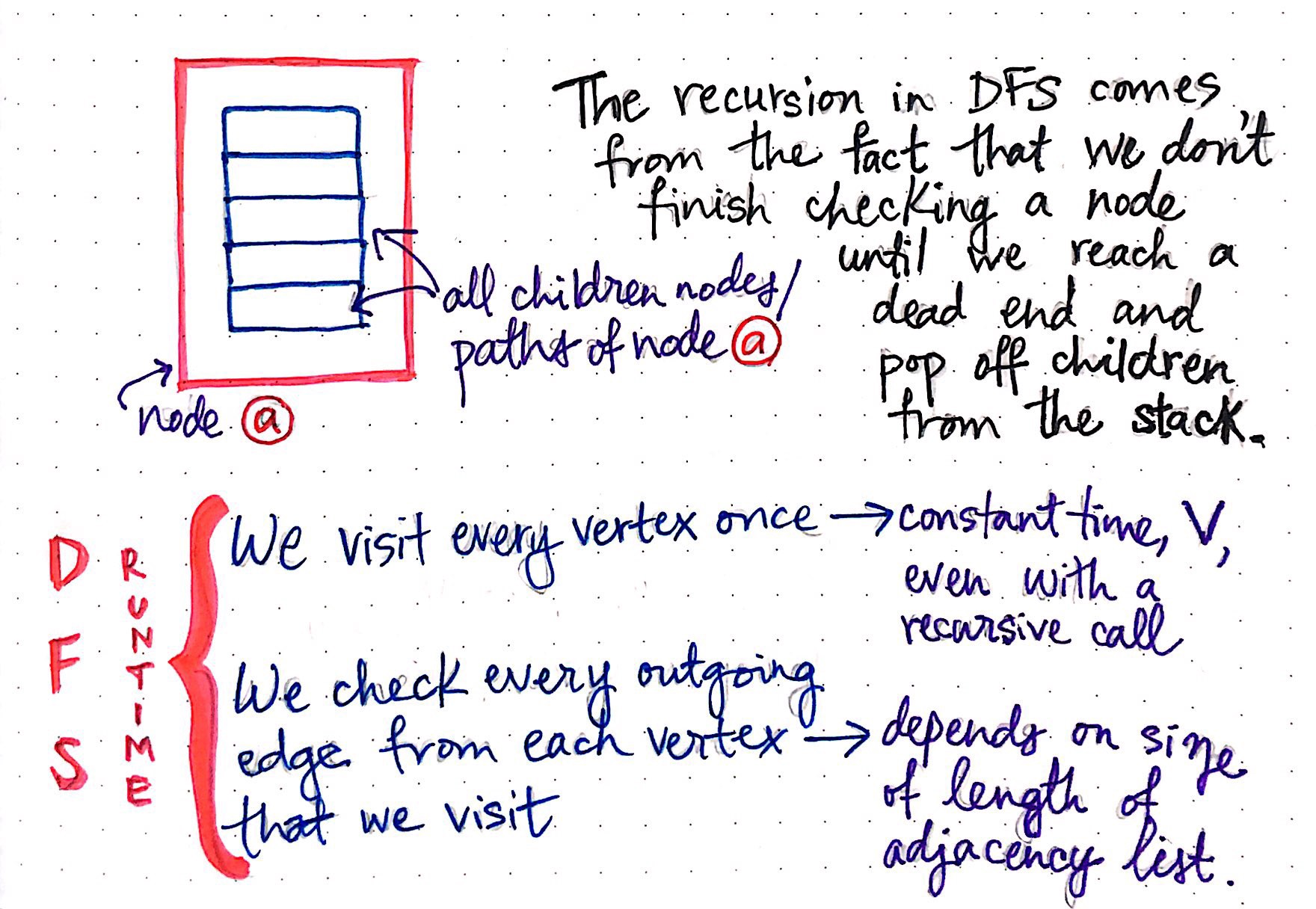
The recursion of the DFS algorithm stems from the fact that we don?t actually finish checking a ?parent? node until we reach a dead end, and inevitably pop off one of the ?parent? node?s children from the top of the stack.
 Recursion as applied to DFS runtime
We can think of the recursive aspect of DFS as a function call to ?visit? a node within another, already-running function call to ?visit? a node. For example, when we begin visiting node a, we are still in the process of visiting node a when we start visiting one of its children, like node c.
And yet, despite the recursion that is built-in to depth-first search, the runtime of this algorithm in real life isn?t actually too terribly affected by the recursive aspect of this graph traversal technique. In fact, even with the recursion, the process of visiting every vertex in the graph once takes constant time. So, if checking a vertex once isn?t the expensive part of this algorithm?then what is?
The answer is lies in the edges ? more specifically, the price of checking the outgoing edges from each vertex that we visit can turn out to be both pretty expensive, and time-consuming. This is because some nodes could have only one neighboring vertex to check, and thus, only one edge, while other nodes could have five, or ten, or many more edges to check! So, really, the runtime of checking every outgoing edge from one vertex to another depends solely upon the size/length of any given node?s adjacency linked list, which is calculated as linear time.
 We could apply DFS in the same way on an undirected graph
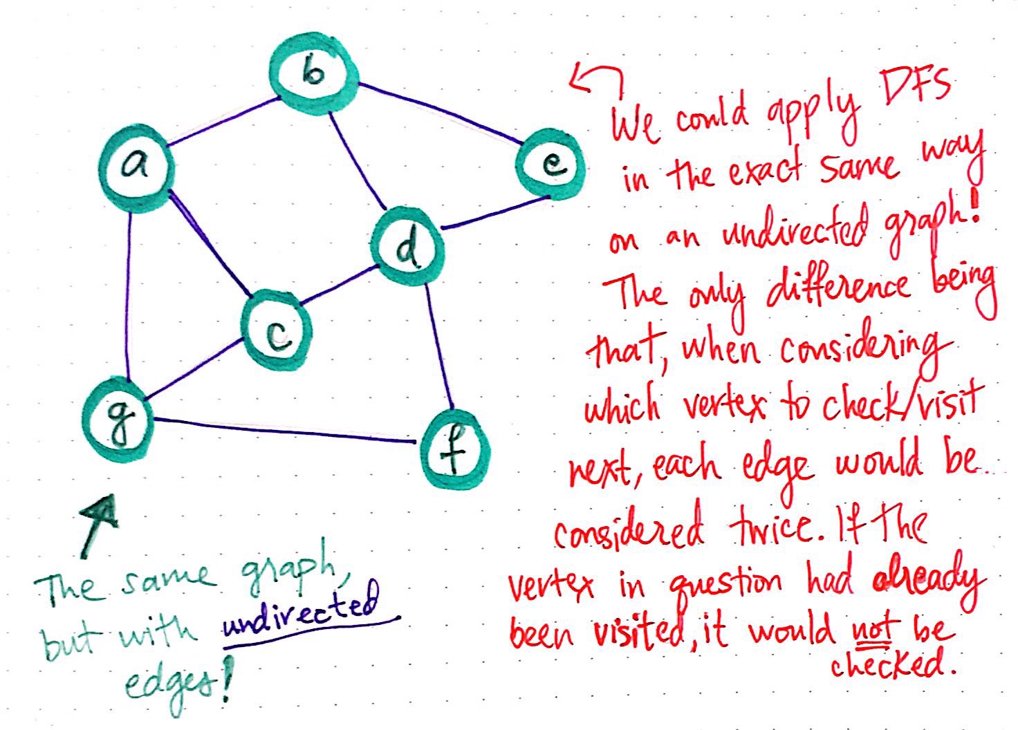
We?ll recall from the basics of graph theory that a graph can have either undirected or directed edges. Just as undirected and directed graphs had slightly different runtimes based on whether the edges appeared once or twice in the adjacency list representation of a graph for breadth-first search, it?s a similar story here, too.
In fact, we could have applied DFS in the exact same way to the same graph we?ve been dealing with, even if it were undirected. The only major difference would have been the fact that, when considering which vertex to ?visit? next while running DFS, each edge in the graph would have been considered twice.
 Depth-first search and linear runtime
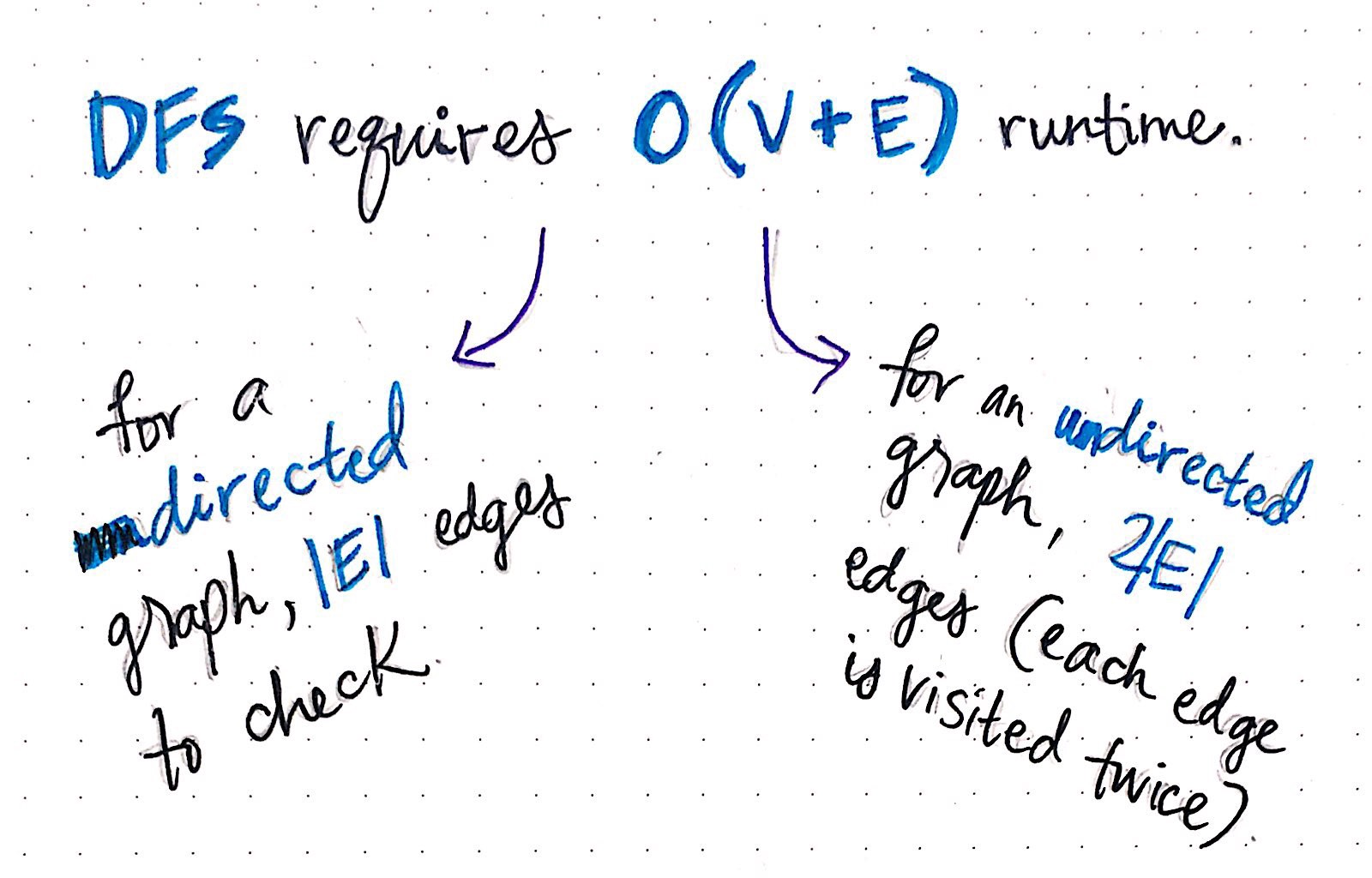
Thus, the actual runtime of DFS is actually no different than that of BFS: they both take linear time, with the slight differentiation being the number of edges (the length of the adjacency linked list) of the graph, based on whether the graph is directed or undirected. For a directed graph, the runtime amounts to a runtime of O(V + |E|), while for an undirected graph, the runtime is calculated as O(V + 2|E|), both of which result in linear time.
But wait ? how does all of this theoretical recursion tie back into the actual implementation of this algorithm? We already know how graphs are represented using adjacency lists. We also know how to use those representations to make sense of other algorithms, like breadth-first search. So how can we make sense of the depth-first algorithm in a similar way?
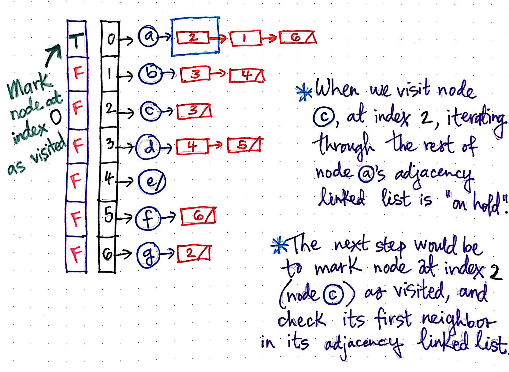
Well, let?s think about what would happen when we run DFS on the adjacency list representation of this same graph. The image below illustrates what that adjacency list might look like.
 Implementing DFS using an adjacency list, Part 1
When we first visit our ?parent? node a, we added it to our stack, and marked it as visited. In the context of our adjacency list, we are marking our ?visited array?, and flagging the index of the vertex we just pushed onto our stack (index 0), marking its ?visited? status as TRUE.
Next, we?ll take a look at the first item in node a’s adjacency linked list. In this case, the first item in the list is a reference to the item at index 2, which is node c. We?ll visit node c next, and, in the process, we?ll put the rest of the work of iterating through node a’s adjacency linked list ?on hold?. In other words, we?re going to look up the node at index 2 next, rather than iterate through the rest of node a’s adjacency linked list and look at whatever element happens to be at index 1.
Since the next step is to mark the node at index 2 as visited, we?ll do exactly that. The vertex at index 2 is node c, so we?ll add it to our stack, mark it as visited, and check its first neighbor in its adjacency linked list. We?ve already gone through these steps previously, so let?s skip to the point where we hit the dead end and have to backtrack back up to the ?parent? node ? that?s where things get interesting!
 Implementing DFS using an adjacency list, Part 2
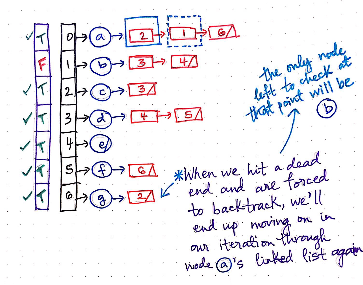
After we?ve traversed down all the way to check and visit node g, we hit a dead end, and backtrack back up to node a, located at index 0. It is only at this point that we pick up where we left off; that is to say, we?ll continue now with the process of iterating through node a’s adjacency linked list (Finally!).
The next element in node a?s adjacency linked list is a reference to the index 1, which is a reference to the vertex b. At this point, we?ll also notice that the entire ?visited? array is marked with TRUE’s everywhere, with only one exception: vertex b. This means that once we check node b and mark it as ?visited?, we will have traversed through the whole graph and voil ? we?re done!
That wasn?t too terrible, was it?
 Depth-first vs breadth-first: pros and cons
The differences between depth-first search and breadth-first search can be subtle at first and tricky to notice at first! They both can be implemented on an adjacency list representation of a graph, and they each result in the same runtime, and involve iterating through the adjacency list of every vertex within a graph. However, there are slight differences in their implementation that we can start to pick up on once we see each of these algorithms in action.
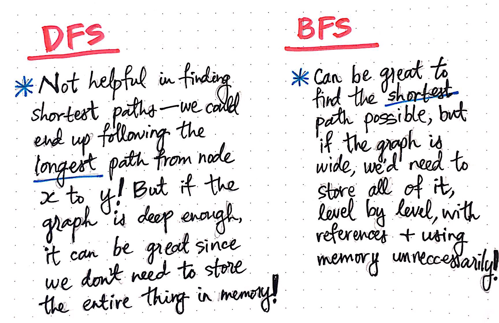
The important thing to remember about both of these algorithms is that neither one is necessarily better than the other. For example, depth-first search is great in determining whether a path exists between two nodes, and doesn?t necessarily require a lot memory, since the entire graph doesn?t need to be initialized or instantiated in order to traverse through it. However, DFS isn?t helpful in finding a shortest path between two nodes; indeed, we might end up inadvertently finding the longest path! In comparison, BFS is great at finding the shortest path between two nodes, but often requires us to store the entire graph as we search through it, level by level, which can cost a lot in space and memory.
Each solution has its benefits and drawbacks. But, they are two different ways of solving a problem and, depending on what kind of problem we have, they might just end up being the perfect tool for the job.
Resources
Depth-first search can be explained and implemented in a few different ways, and trying to understand all of them ? at least, when you?re first learning the DFS algorithm ? can feel overwhelming. However, once you?re more comfortable and familiar with how it works, it?s helpful to know the different implementations and idiosyncrasies of how DFS works. If you?re looking to gain a deeper understanding of this algorithm, here are some good examples and implementations to help you get started.
- Depth-first Search (DFS) on Graphs Part 2, Sesh Venugopal
- Depth-First Search, Department of Computer Science, Harvard
- When is it practical to use DFS vs BFS?, StackOverflow
- Depth-First Search (DFS), Topological Sort, MIT OpenCourseWare
- Graph Traversals ? Breadth First and Depth First, CollegeQuery
