
Finding the paths ? and especially the shortest path ? between two nodes is a well studied problem in graph theory. This is because paths in a graph are frequently an interesting property. In the three jugs problem a path from the start node to any node with 6 liters of water in one jug represented a solution to the riddle. In a social network a path might show us how two people are connected, the length of the shortest path between two people might tell us something about the social distance between them. In a graph representing roadways the shortest path between two nodes might very literally represent the shortest path between two places.
In an upcoming section we will implement both of these algorithms in Python. Before we do that, we will have to implement a simple graph API, also in Python. But before we do either of those we are going to define BFS and DFS at a higher level ? as a process that we can apply to graphs in the abstract, without worrying about pesky implementation details.
Breadth first search (BFS) and Depth First Search (DFS) are the simplest two graph search algorithms. These algorithms have a lot in common with algorithms by the same name that operate on trees. If you have studied trees before, a lot of this will section will be a review, and if you have not, then by the end of this section you?ll know two tree algorithms as well as two graph algorithms.
The crucial difference between trees and graphs (which creates a difference in the DFS/BFS implementation) is that in trees there are no cycles. In graph theory, a cycle exists in any graph where you can leave a node and travel through the graph back to that node. Undirected graphs always contain cycles because you can simple go back and forth between any two neighbors. There is one exception to that rule: a graph with no edges. On the other hand, such a graph is rather boring, and probably not worth studying.
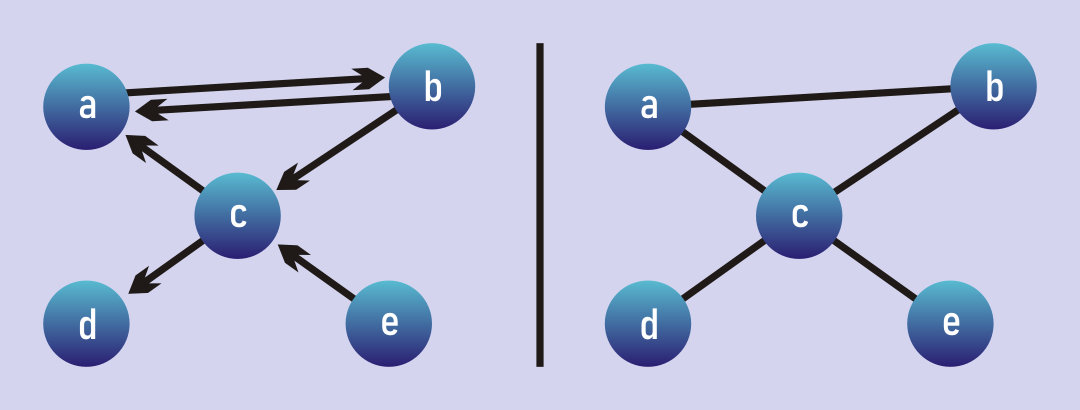 Both graphs contain multiple cycles. Left: a,b,a and a,b,c,a. Right: any 2 node pair, a,b,c,a, d,c,b,a,c,d? and more.
In a directed graph, you might or might not have cycles. Directed graphs without cycles are called Directed Acyclic Graphs (DAGs) and have a number of special properties and special algorithms that exploit those properties. For now though, what?s important is that our two search algorithms have to account for cycles so that they don?t get caught in an infinite loop. Supposed we wanted to find a path from d to e the undirected graph above. Our algorithm has to be smart enough to avoid searching from d to c to b to a to c then back to b. It?s not terribly hard to do, but it is important.
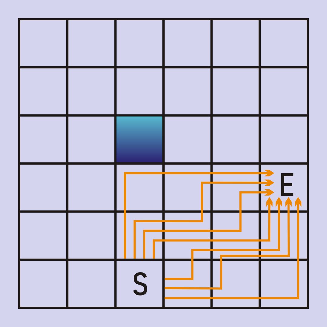
BFS and DFS are both simple algorithms, and they are quite similar. With both algorithms, we explore individual nodes ? one by one ? until we find a node matching a particular condition. For example, in the 3 Jugs Problem the condition is that one of the jugs has 6 gallons of water in it. In Google Maps the condition is that we find the node representing a specific place. For the rest of this section, we?re going to model a 2D maze as a graph to help us explore graph search. Here is our simple maze:
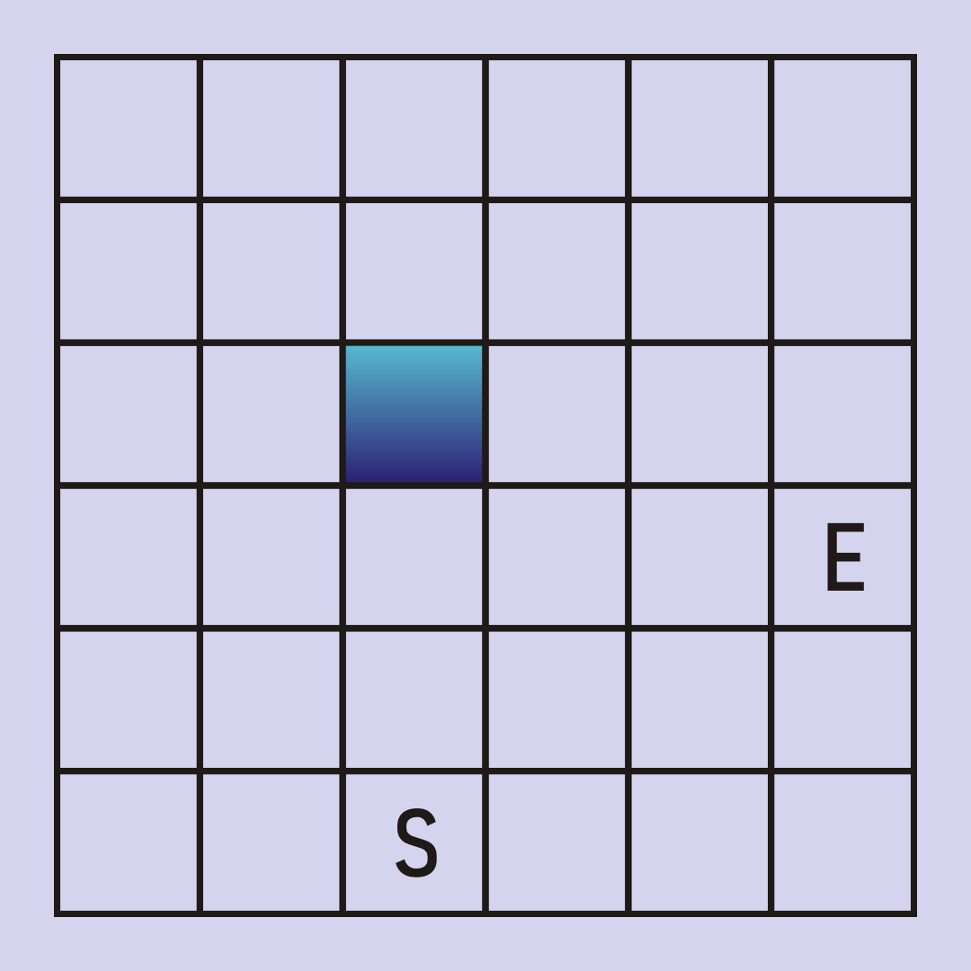 S for Start, E for End.
Obviously, this is a very simple maze ? it?s simplicity will help us focus on graph search. Our maze has a start cell, an end cell, many empty cells, and some walls represented by filled in cells. As a graph, each empty square is a node and has edges only to the nodes above, below, left, and right of it. Filled in squares are walls and are left out of the graph entirely. This means any node will have a maximum of 4 edges with nodes on the side or next to walls having fewer edges. The goal of graph search in this problem is to find a path from the start node to the end node, ideally the shortest such path.
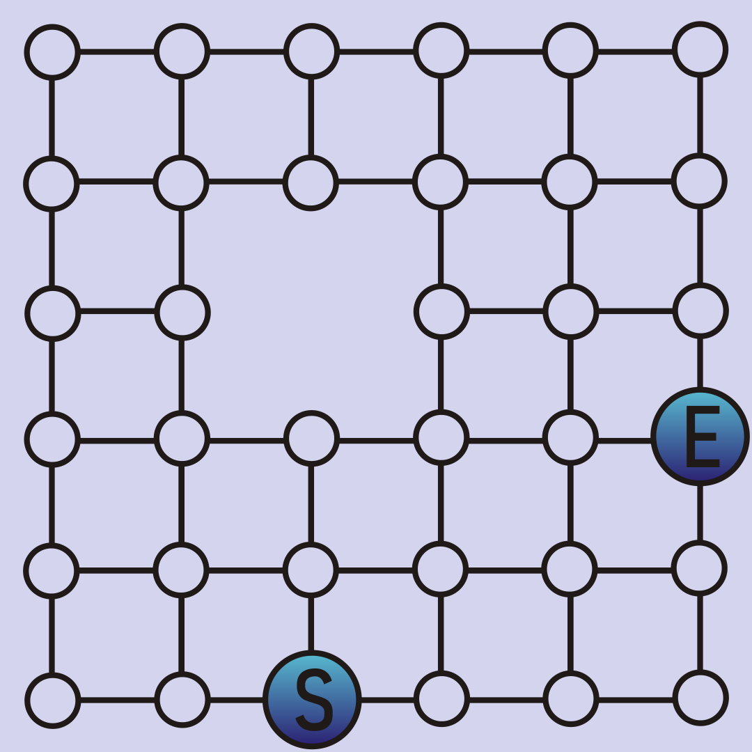
Here is our maze in a nodes and edges representation:
Depth First Search
Depth first search is dead simple. First, go to the specified start node. Now, arbitrarily pick one of that node?s neighbors and go there. If that node has neighbors, arbitrarily pick one of those and go there unless we?ve already seen that node. And we just repeat this process until one of two things happens. If reach the specified end node we terminate the algorithm and report success. If we reach a node with only neighbors we?ve already seen, or no neighbors at all, we go back one step and try one of the neighbors we didn?t try last time.
This algorithm is called depth first search because we always prioritize searching the deepest node we know about. If there are ties, they are broken arbitrarily, but once we break our first tie (picking which neighbor of the start node to explore first) we will not try to search the other neighbors of the start_node until the first neighbor (and all of its neighbors) have been fully explored.
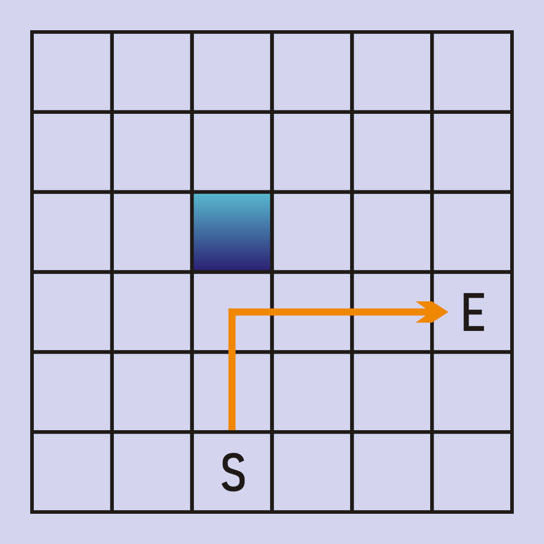
Consider our maze, and a DFS implementation that breaks ties by searching up first, then right, then left, then right. Our algorithm will go straight up until it hits a wall, then straight to the right to arrive at our end node.
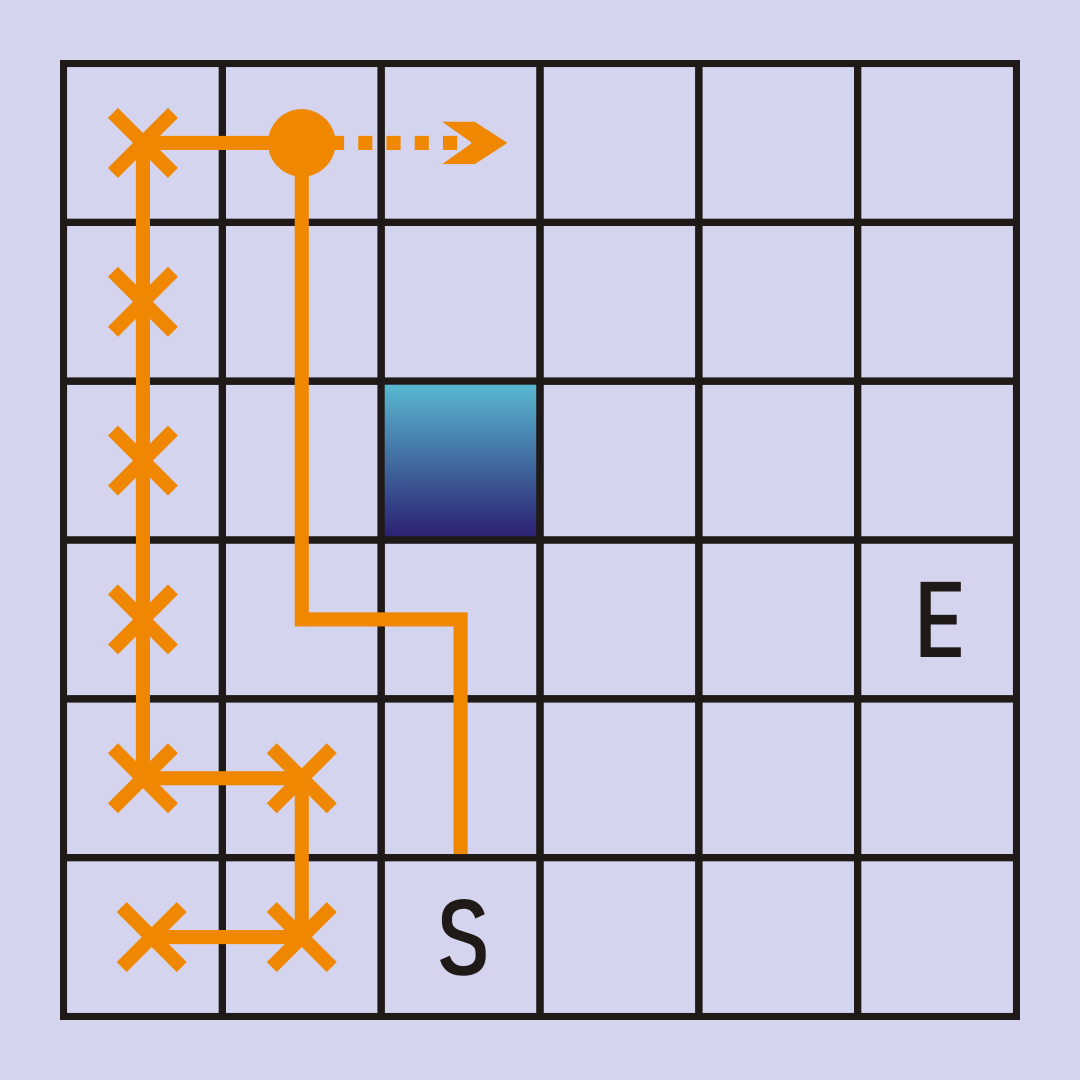
Now, consider an implementation of DFS where ties are broken by searching up, then left then right, then down. Now we?ll search nodes in a very inefficient pattern, and reach a point where the algorithm has to backtrack and simulate a different decision in order to find a path to the goal.
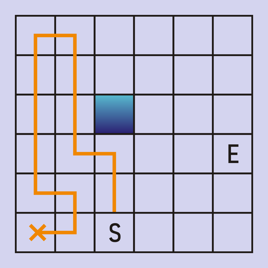
In this specific case we will backtrack repeatedly. All of the squares with an orange line through it are ?explored? already ? we have to backtrack until we reach a node with at least one unexplored neighbor.
If we were to follow this instance of DFS all the way to it?s completion (remember, ties are broken up, left, right, down) the path we?d ultimately find looks like this:
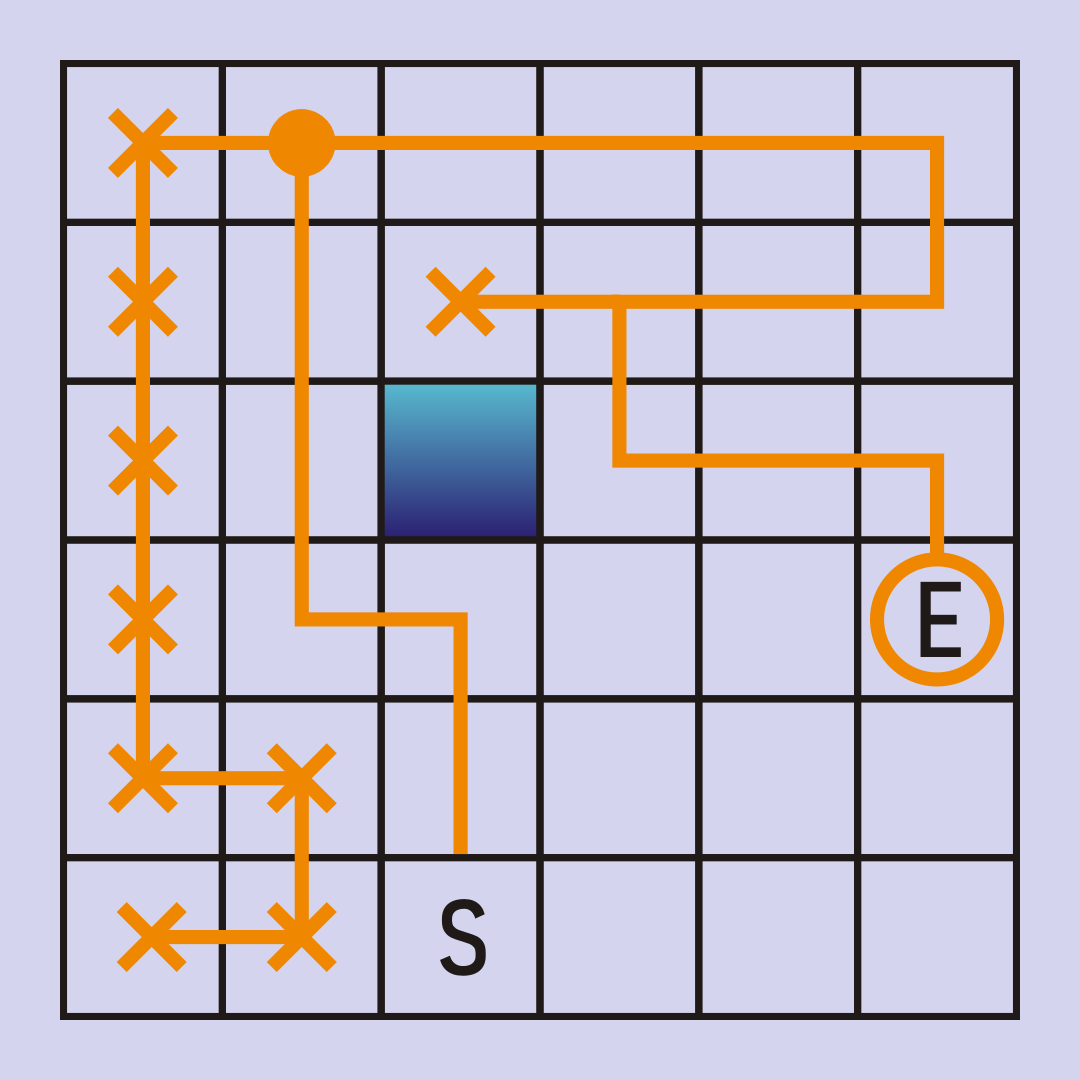
After backtracking one more time, just above the wall, we find the end node. This time around we processed more nodes and found a much longer path from start to end. This illustrates an important point about DFS: while it is sure to find a path if a path exists, it is not sure to find the shortest path.
To implement these two algorithms, we need to define two terms, the frontier and the explored list. The frontier is the list of nodes we know about, but have not visited. The explored list is the list of nodes that we?ve already visited. We use the frontier to track of which nodes will be explored next ? the ordering of the frontier controls which search algorithm we?re performing. The explored list is used to prevent us from searching nodes we?ve already explored ? and thus prevents us from searching in an infinite loop if there are cycles.
Because there might be multiple paths to any particular node, the frontier may end up with multiple entries for a single node. The explored list, however, will always contain only one entry per node ? once we explore a node we ignore it if we encounter it again in the future. Thus the explored list is actually a set. To be ?explored? a node simply needs to have had all of its children added to the frontier.
Here is DFS in pseudocode:
DFS(graph, start_node, end_node): frontier = new Stack() frontier.push(start_node) explored = new Set() while frontier is not empty: current_node = frontier.pop() if current_node in explored: continue if current_node == end_node: return success for neighbor in graph.get_neigbhors(current_node): frontier.push(neighbor) explored.add(current_node)
There are two things to note about this code. 1) There is no ?backtracking? step making itself obvious. Instead, backtracking occurs in the form of popping nodes off of the frontier. 2) The use of a stack for the frontier ensures that nodes are searched in a depth first ordering, since the most recently added node will always be explored next.
Breadth First Search
The only difference between DFS and BFS is the order in which nodes are processed. In DFS we prioritized the deepest node in the frontier, in BFS we do the opposite. We explore all the neighbors of our starting node before exploring any other node. After we have explored all the immediate neighbors we explore nodes that are 2 hops away from the starting node. Then 3 hops, then 4 hops, and so on.
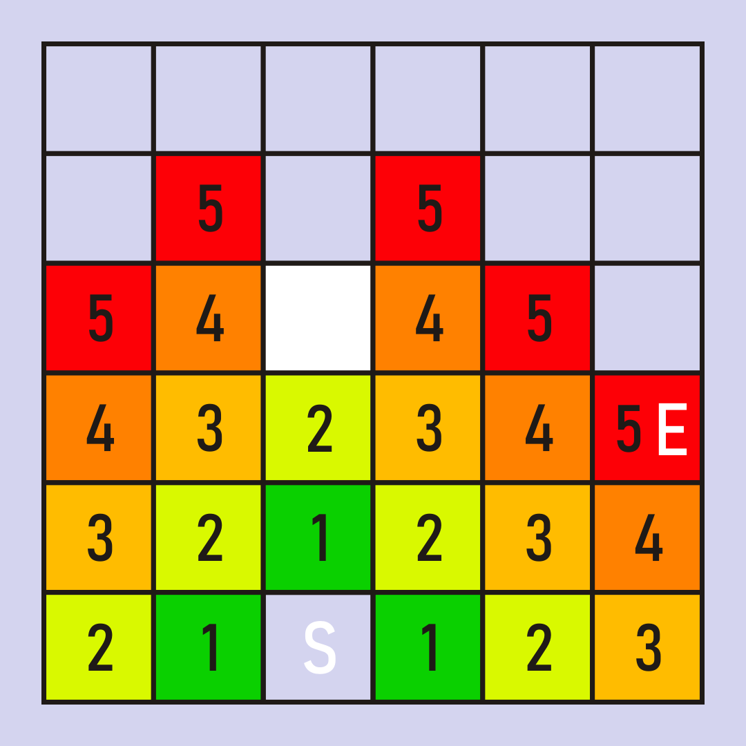
Notice how the frontier expands like a ripple in a pond ? first the 1?s are added. By processing all the 1?s, all the 2?s are added to the frontier, and so on. Tie breaking still has an impact, for example all of the 5?s might be processed, but if our tiebreaking strategy causes the end node to be processed as the first of the 5?s then it would be the only 5 explored. Also note that there are several possible paths of length 5 from the start to the end in this maze; the tie breaking mechanism will determine which of these paths is ultimately found:
This example illustrates another difference between DFS and BFS. In DFS we?d search along a single path, then ?backtrack? when we reach a dead end. With BFS we?re not really exploring along a path, instead we?re exploring along several possible paths at once. When one reaches a dead end, we just stop searching in that direction and focus on whatever else is in the frontier.
Finally, if the graph is unweighted BFS will always find the shortest path. This is in contrast to DFS which provides no guarantees about the length of the path it finds. Showing that BFS always finds the shortest path is fairly straightforward ? all the paths of length 1 will be searched before any of the paths of length 2. If the shortest path is length 1, then it must be found before any path of length 2 is even considered.
The pseudocode for BFS is remarkably close to DFS, the only difference is that the frontier is a queue instead of a stack.
BFS(graph, start_node, end_node): frontier = new Queue() frontier.enqueue(start_node) explored = new Set() while frontier is not empty: current_node = frontier.dequeue() if current_node in explored: continue if current_node == end_node: return success for neighbor in graph.get_neigbhors(current_node): frontier.enqueue(neighbor) explored.add(current_node)
Although it?s possible to say much more about graphs in the abstract, it is more helpful to balance our theory with implementation. In the next section we will explore a few different ways to implement a graph, then we?ll select one of these and actually implement it in Python.
Once we have an implementation of a graph API that we?ll implement BFS and DFS for that API, and use our implementations to solve some problems.
Next article in the series: Graph Implementations
Table of contents

