The last few days I have been thinking a lot about different ways of measuring correlations between variables and their pros and cons. Here?s the problem: there are two kinds of variables ? continuous and categorical (sometimes called discrete or factor variables) and hence, we need a single or different metrics which can quantify correlation or association between continuous-continuous, categorical-categorical and categorical-continuous variable pairs. Computing correlation can be broken down into two sub-problems ? i). Testing if there is a statistically significant correlation between two variables and ii). Quantifying the association or ?goodness of fit? between the two variables. Ideally, we also need to be able to compare such goodness of fit metrics between variable pair classes on some universal scale. This problem becomes important if the matrix you are analyzing has a combination of categorical and continuous variables. In these cases, if you want a universal criterion to drop columns above a certain correlation from further analyses, it is important that all correlations computed are comparable. There is no single technique to correlate all the three variable pairs and so having such a universal scale for comparing correlations obtained from different methods is tricky and needs some thinking.
You might be wondering why anyone would ever need to compare correlation metrics between different variable types. In general, knowing if two variables are correlated and hence substitutable is useful for understanding variance structures in data and feature selection in machine learning. To expand, for data exploration and hypothesis testing, you want to be able to understand the associations between variables. Additionally, for building efficient predictive models, you would ideally only include variables that uniquely explain some amount of variance in the outcome. In all these applications, it is likely that you will be comparing correlations between continuous, categorical and continuous-categorical pairs with each other and hence having a shared estimate of association between variable pairs is essential. One thing to note is that for all these applications while a statistical significance test of correlation between the two variables is helpful, it is far more important to quantify the association in a comparable manner i.e. have a comparabale ?goodness of fit? metric.
I was surprised that I did not find a comprehensive overview detailing correlation measurement between different kinds of variables, especially goodness of fit metrics, so I decided to write this up.
There has been a lot of focus on calculating correlations between two continuous variables and so I plan to only list some of the popular techniques for this pair. Out of these three variable combinations, computing correlation between a categorical-continuous variable is the most non-standard and tricky. Surprisingly (or may be not so much), there is very little formal literature on correlating such variables. Hence, I plan to spend most parts of this post expanding on standard and non-standard ways to calculate such correlations. Finally, with the rise of categorical variables in datasets, it is important to calculate correlations between this pair of variables (i.e., a categorical and another categorical variable). Let us start with a discussion surrounding computing correlation between two categorical variables.
Correlation between two discrete or categorical variables
Broadly speaking, there are two different ways to find association between categorical variables. One set of approaches rely on distance metrics such as Euclidean distance or Manhattan distance while another set of approaches span various statistical metrics such as chi-square test or Goodman Kruskal?s lambda, which was initially developed to analyze contingency tables. Now the mathematical purist out there could correctly argue that distance metrics cannot be a correlation metric since correlation needs to be unit independent which distance by definition can?t be. I do agree with that argument and I will point it out later but for now I include it since many people use distance as a proxy for correlation between categorical variables. Additionally, in certain special situations there is an easy conversion between Pearson correlation and Euclidean distance.
Below, I list some common metrics within both approaches and then discuss some relative strengths and weaknesses of the two broad approaches. Then, I list some commonly used metrics within both approaches and end with a brief discussion of their relative merits.
Distance Metrics
Although the concept of ?distance? is often not synonymous with ?correlation,? distance metrics can nevertheless be used to compute the similarity between vectors, which is conceptually similar to other measures of correlation. There are many other distance metrics, and my intent here is less to introduce you to all the different ways in which distance between two points can be calculated, and more to introduce the general notion of distance metrics as an approach to measure similarity or correlation. I have noted ten commonly used distance metrics below for this purpose. If you are interested in learning more about these metrics, definitions and formulas can be found here.
- Sum of Absolute Distance
- Sum of Squared Distance
- Mean-Absolute Error
- Euclidean Distance
- Manhattan Distance
- Chessboard Distance
- Minkowski Distance
- Canberra Distance
- Cosine Distance
- Hamming Distance
Contingency Table Analysis
When comparing two categorical variables, by counting the frequencies of the categories we can easily convert the original vectors into contingency tables. For example, imagine you wanted to see if there is a correlation between being a man and getting a science grant (unfortunately, there is a correlation but that?s a matter for another day). Your data might have two columns in this case ? one for gender which would be Male or Female (assume a binary world for this case) and another for grant (Yes or No). We could take the data from these columns and represent it as a cross tabulation by calculating the pair-wise frequencies
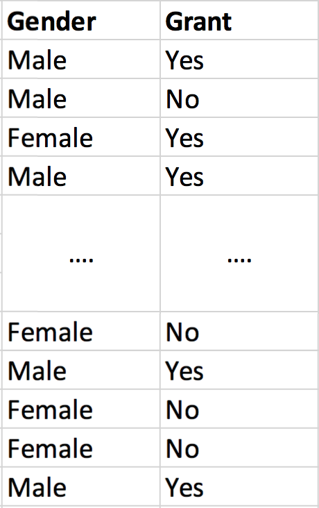 Original data table with two columns having some categorical data
 Cross Tabulating the categorical variables and presenting the same data as a contingency table
Contingency tables or cross tabulation display the multivariate frequency distribution of variables and are heavily used in scientific research across disciplines. Due to their heavy historic use in statistical analyses, a family of tests have been developed to determine the significance of the difference between two categories of a variable compared to another categorical variable. A popular approach for dichotomous variables (i.e. variables with only two categories) is built on the chi-squared distribution. We are not interested in testing the statistical significance however, we are more interested in effect size and specifically in the strength of association between the two variables. Thankfully, several coefficients have been defined for this purpose, including several which use the chi-square statistic. Here are some examples:
- Goodman Kruskal?s lambda
- Phi co-efficient (uses chi-squared statistic)
- Cramer?s V (uses chi-squared statistic)
- Tschuprow?s T (uses chi-squared statistic)
- Contingency coefficient C (uses chi-squared statistic)
Relative strengths and weaknesses
Distance metrics, at least to me, are more intuitive and easier to understand. It makes sense that if one variable is perfectly predictive of another variable, when plotted in a high dimensional space, the two variables will overlay or be very close to each other. Since I believe that methods one uses to analyze data be easily explainable to non-statisticians whenever possible , using distance has an obvious appeal. But a big drawback of approaches relying on distance metrics is that they are scale dependent. If you scale your input by a factor of 10, any distance metric will be sensitive to it and change significantly. This behavior is obviously not desirable to understand goodness of fit between different features. Additionally, distance metrics are not easily comparable between variable pairs with different number of categories. Let me illustrate this with an example ? let?s say we have 3 columns ? gender with two categories (Male represented by 0 and Female represented by 1), grades with three categories (Excellent represented by 2, Good represented by 1 and Poor represented by 0) and college admission (Yes represented by 1 and No represented by 0). We want to compare whether gender is more correlated with college admission or grades are more correlated with college admission. Since, the values of grades range from [0, 2] while gender ranges from [0,1] the distance between college admission (range ? [0,1]) and grades will be artificially inflated compared to the distance between college admission and gender. This problem can be easily removed though if you one-hot encode all variables in your matrix before computing correlations such that every categorical variable will only have two values ? Yes (1) or No (0).
Another potentially bigger drawback of using distance metrics is that sometimes there isn?t a straightforward conversion of a distance metric into a goodness of fit coefficient which is what we want we are more interested in for the purposes of this blog post. I should note here that if you scale and center your continuous data, Euclidean distance could still be used since in these cases there is an easy conversion of Euclidean distance to Pearson correlation. Of course, the other solution one could try would be to use different cutoff criteria for correlations between two discrete variables compared to two continuous variables. But, according to me that is not ideal since we want a universal scale to compare correlations between all variable pairs.
Although statistical techniques based on analyzing contingency tables suffer from fewer drawbacks compared to distance metrics, there are nonetheless important issues which mostly arise from how the statistical significance test (for example: chi-square statistic) is converted into a measure of association. Some of the coefficients such as Phi are defined only for 2×2 tables. Additionally, the contingency coefficient C suffers from the disadvantage that it does not reach a maximum value of 1. The highest value of C for a 2×2 table is 0.707 and for a 4×4 table it is 0.870. This means that C cannot be used to compare associations among tables with different numbers of categories or in tables with a mix of categorical and continuous variables. Further, other measures such as Cramer?s V can be a heavily biased estimator, especially compared to correlations between continuous variables and will tend to overestimate the strength of the association. One way to mitigate the bias in Cramer?s V is to use a kind of bias correction suggested here. The bias corrected Cramer?s V shown to typically have a much smaller mean square error.
Correlation between a continuous and categorical variable
Out of all the correlation coefficients we have to estimate, this one is probably the trickiest with the least number of developed options. There are three big-picture methods to understand if a continuous and categorical are significantly correlated ? point biserial correlation, logistic regression, and Kruskal Wallis H Test.
Point biserial Correlation
The point biserial correlation coefficient is a special case of Pearson?s correlation coefficient. I am not going to go in the mathematical details of how it is calculated, but you can read more about it here. I will highlight three important points to keep in mind though:
- Similar to the Pearson coefficient, the point biserial correlation can range from -1 to +1.
- The point biserial calculation assumes that the continuous variable is normally distributed and homoscedastic.
- If the dichotomous variable is artificially binarized, i.e. there is likely continuous data underlying it, biserial correlation is a more apt measurement of similarity. There is a simple formula to calculate the biserial correlation from point biserial correlation, but nonetheless this is an important point to keep in mind.
Logistic Regression
The idea behind using logistic regression to understand correlation between variables is actually quite straightforward and follows as such: If there is a relationship between the categorical and continuous variable, we should be able to construct an accurate predictor of the categorical variable from the continuous variable. If the resulting classifier has a high degree of fit, is accurate, sensitive, and specific we can conclude the two variables share a relationship and are indeed correlated.
There are a number of positive things about this approach. Logistic regression does not make many of the key assumptions of linear regression and other models that are based on least squares algorithms ? particularly regarding linearity, normality, homoscedasticity, and measurement level. However, I should note here logistic regression does assume that there is a linear relationship between the predictors and the logit of the outcome variable and often times not only is this assumption invalid, it is also not straightforward to verify. I would advise the user to keep this in mind before using logistic regression. On the positive side, since we only have one feature for prediction, there is no problem of multicollinearity similar to other applications of logistic regression.
Kruskal-Wallis H Test (Or parametric forms such as t-test or ANOVA) ? Estimate variance explained in continuous variable using the discrete variable
The final family of methods to estimate association between a continuous and discrete variable rely on estimating the variance of the continuous variable, which can be explained through the categorical variable. There are many ways to do this. A simple approach could be to group the continuous variable using the categorical variable, measure the variance in each group and comparing it to the overall variance of the continuous variable. If the variance after grouping falls down significantly, it means that the categorical variable can explain most of the variance of the continuous variable and so the two variables likely have a strong association. If the variables have no correlation, then the variance in the groups is expected to be similar to the original variance.
Another approach which is more statistically robust and supported by a lot of theoretical work is using one-way ANOVA or its non-parametric forms such as the Kruskal-Wallis H test. A significant Kruskal?Wallis test indicates that at least one sample stochastically dominates another sample. The test does not identify where this stochastic dominance occurs or for how many pairs of groups stochastic dominance obtains. For analyzing the specific sample pairs for stochastic dominance in post hoc testing, Dunn?s test, pairwise Mann-Whitney tests without Bonferroni correction, or the more powerful but less well-known Conover?Iman test are appropriate or t-tests when you use an ANOVA?might be worth calling that out. Since it is a non-parametric method, the Kruskal?Wallis test does not assume a normal distribution of the residuals, unlike the analogous one-way analysis of variance. I should point out that though ANOVA or Kruskal-Wallis test can tell us about statistical significance between two variables, it is not exactly clear how these tests would be converted into an effect size or a number which describes the strength of association.
Relative Strengths and Weaknesses
The point biserial correlation is the most intuitive of the various options to measure association between a continuous and categorical variable. It has obvious strengths ? a strong similarity with Pearson correlation and is relatively computationally inexpensive to compute. On the downside, it makes strong assumptions about data regarding normality and homoscedasticity. Additionally, similar to the Pearson correlation (read more details in the next section), it is only useful in capturing somewhat linear relationships between the variables. Of course, for many data science applications these assumptions are too restrictive and make point biserial an unsuitable choice in those situations.
Logistic regression aims to alleviate many of the problems of using a point biserial correlation. I am not going to go into all the theoretical advantages of logistic regression here, but I want to highlight that logistic regression is more robust mainly because the continuous variables don?t have to be normally distributed or have equal variance in each group. Additionally, it can also help us model and detect non-linear relationships between the categorical and continuous variables. But that are a few downsides to logistic regression as well. One big issue is that logistic regression, like many other classifiers, is sensitive to class imbalances i.e. if you have 100 0?s and only 10 1?s in your dataset, logistic regression may not build a great classifier. The other issue is that a pseudo R-squared is calculated by many logistic regression algorithms, but these should be interpreted with extreme caution as they have many computational issues which cause them to be artificially high or low. One simple approach would be to take some sort of weighted average of pseudo R-squared reported by different methods.
Correlation between two continuous variables
Correlating two continuous variables has been a long-standing problem in statistics and so over the years several very good measurements have been developed. There are two general approaches for understanding associations between continuous variables ? linear correlations and rank based correlations.
Linear Association (Pearson Correlation)
Pearson correlation is one of the oldest correlation coefficients developed to measure and quantify the similarity between two variables. Formally, Pearson?s correlation coefficient is the covariance of the two variables divided by the product of their standard deviations. The form of the definition involves a ?product moment?, that is, the mean (the first moment about the origin) of the product of the mean-adjusted random variables; hence the modifier product-moment in the name. I don?t see great reason for going in more detail about it since there is extensive information about it on the internet, but I will point out a few assumptions and limitations though.
- Strong influence of outliers ? Pearson is quite sensitive to outliers
- Assumption of linearity ? The variables should be linearly related
- Assumption of homoscedasticity
In light of these assumptions, I suggest it would be best to make a scatter plot of the two variables and inspect these properties before using Pearson?s correlation to quantify the similarity. While this is general advice which should always be followed, I believe it is extra critical if you plan to use Pearson as a measure of correlation.
Ordinal Association (Rank correlation)
Often, we are interested in understanding association between variables which may be related through a non-linear function. In these cases, even when variables have a strong association, Pearson?s correlation would be low. To properly identify association between variables with non-linear relationships, we can use rank-based correlation approaches. Below there are four examples of ordinal or rank correlation approaches:
- Spearman Correlation
- Goodman Kruskal?s Gamma
- Kendall?s Tau
- Somers? D
I am not going to go into greater detail on the relative strengths and weaknesses of ordinal association versus linear association. The matter has been extensively discussed elsewhere. I will highlight the main difference because it is important to keep this in mind ? Pearson correlation is only helpful in detecting linear relationships and for detecting other relationships rank-based approaches such as Spearman?s correlation should be used. In practice, I default to using Spearman?s correlation anytime I have to correlate two continuous variables.
Summary
When I started thinking about calculating pairwise correlations in a matrix with several variables ? both categorical and continuous, I believed it was an easy task and did not imagine of all the factors which could confound my analysis. Additionally, I did not find a comprehensive overview of the different measures I could use. There are mainly three considerations which we need to balance in deciding which metric to use:
- Are you looking to detect only linear relationships between your variables which are normally distributed and homoscedastic?
- What is the size of the dataset you are working with?
- Do you eventually plan on comparing the correlation between different variables; may be drop the variables which are highly correlated?
In most applications, it makes sense to use a bias corrected Cramer?s V to measure association between categorical variables. Methods such as Pearson correlation and point biserial correlation are really inexpensive to implement and provide excellent correlation metrics for continuous-continuous and categorical-continuous tests if you have a small dataset with linear relationships between normally distributed and homoscedastic variables. If your application is feature selection for machine learning and you have a large dataset, I would suggest using logistic regression to understand association between categorical and continuous variable pairs and rank-based correlation metrics such as Spearman to understand association between continuous variables.
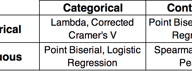
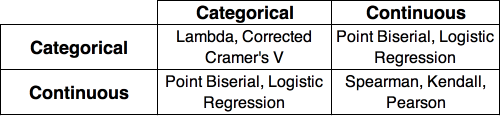 Which correlation metric should you use?

