AlexNet famously won the 2012 ImageNet LSVRC-2012 competition by a large margin (15.3% VS 26.2% (second place) error rates). Here we have a look at the details of the neuron architecture from the related paper ImageNet Classification with Deep Convolutional Neural Networks.
The highlights of the paper
- Use Relu instead of Tanh to add non-linearity. It accelerates the speed by 6 times at the same accuracy.
- Use dropout instead of regularisation to deal with overfitting. However the training time is doubled with the dropout rate of 0.5.
- Overlap pooling to reduce the size of network. It reduces the top-1 and top-5 error rates by 0.4% and 0.3%, repectively.
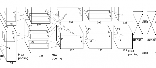
The architecture
It contains 5 convolutional layers and 3 fully connected layers. Relu is applied after very convolutional and fully connected layer. Dropout is applied before the first and the second fully connected year. The image size in the following architecutre chart should be 227 * 227 instead of 224 * 224, as it is pointed out by Andrei Karpathy in his famous CS231n Course. More insterestingly, the input size is 224 * 224 with 2 padding in the pytorch torch vision. The output width and height should be (224?11+4)/4 + 1=55.25! The explanation here is pytorch Conv2d apply floor operator to the above result, and therefore the last one padding is ignored.
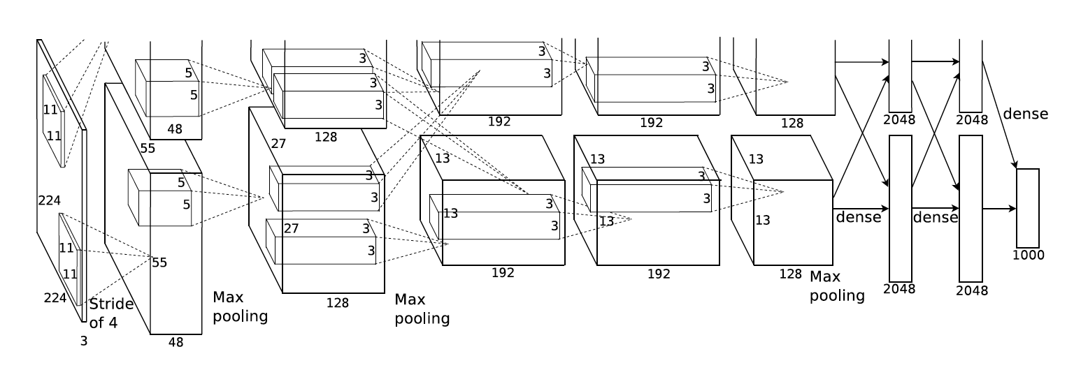 Architecture for the paper
The following table shows different layers, parameters and computation units needed.
AlexNet Architecture
The network has 62.3 million parameters, and needs 1.1 billion computation units in a forward pass. We can also see convolution layers, which accounts for 6% of all the parameters, consumes 95% of the computation. This leads Alex?s another paper, which utilises this feature to improve performance. The basic idea of that paper is as follows if you are interested:
- Copy convolution layers into different GPUs; Distribute the fully connected layers into different GPUs.
- Feed one batch of training data into convolutional layers for every GPU (Data Parallel).
- Feed the results of convolutional layers into the distributed fully connected layers batch by batch (Model Parallel) When the last step is done for every GPU. Backpropogate gradients batch by batch and synchronize the weights of the convolutional layers.
Obviously, it takes advantage of the features we talked above: convolutional layers have a few parameters and lots of computation, fully connected layers are just the opposite.
Training
The network takes 90 epochs in five or six days to train on two GTX 580 GPUs. SGD with learning rate 0.01, momentum 0.9 and weight decay 0.0005 is used. Learning rate is divided by 10 once the the accuracy plateaus. The leaning rate is descreased 3 times during the training process.
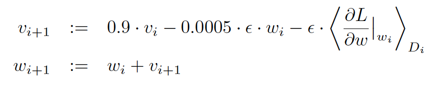 Parameter Updates
Example of implementation
Pytorch has one of the simplest implementation of AlexNet. The architecure follows Alex?s following paper of Alexnet, which doesn?t have normalisation layers, as they don?t improve accuracy. Normalization is not common anymore actually.

