
The method of Lagrange multipliers is the economist?s workhorse for solving optimization problems. The technique is a centerpiece of economic theory, but unfortunately it?s usually taught poorly.
Most textbooks focus on mechanically cranking out formulas, leaving students mystified about why it actually works to begin with. In this post, I?ll explain a simple way of seeing why Lagrange multipliers actually do what they do ? that is, solve constrained optimization problems through the use of a semi-mysterious Lagrangian function.
Some Background
Before you can see why the method works, you?ve got to know something about gradients. For functions of one variable there is ? usually ? one first derivative. For functions of n variables, there are n first derivatives. A gradient is just a vector that collects all the function?s partial first derivatives in one place.
Each element in the gradient is one of the function?s partial first derivatives. An easy way to think of a gradient is that if we pick a point on some function, it gives us the ?direction? the function is heading. If our function is labeled
![]()
the notation for the gradient of f is
![]()
The most important thing to know about gradients is that they always point in the direction of a function?s steepest slope at a given point. To help illustrate this, take a look at the drawing below. It illustrates how gradients work for a two-variable function of x1 and x2.
The function f in the drawing forms a hill. Toward the peak I?ve drawn two regions where we hold the height of f constant at some level a. These are called level curves of f, and they?re marked f = a1, and f = a2.
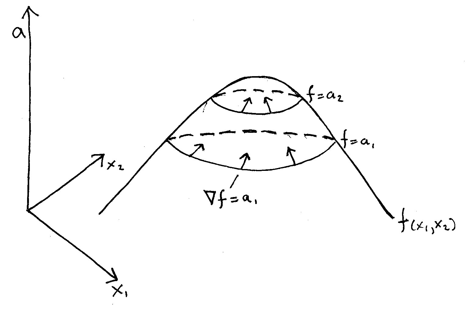
Imagine yourself standing on one of those level curves. Think of a hiking trail on a mountainside. Standing on the trail, in what direction is the mountain steepest? Clearly the steepest direction is straight up the hill, perpendicular to the trail. In the drawing, these paths of steepest ascent are marked with arrows. These are the gradients
![]()
at various points along the level curves. Just as the steepest hike is always perpendicular to our trail, the gradients of f are always perpendicular to its level curves.
That?s the key idea here: level curves are where
![]()
and
![]()
How the Method Works
To see how Lagrange multipliers work, take a look at the drawing below. I?ve redrawn the function f from above, along with a constraint g = c. In the drawing, the constraint is a plane that cuts through our hillside. I?ve also drawn a couple level curves of f.
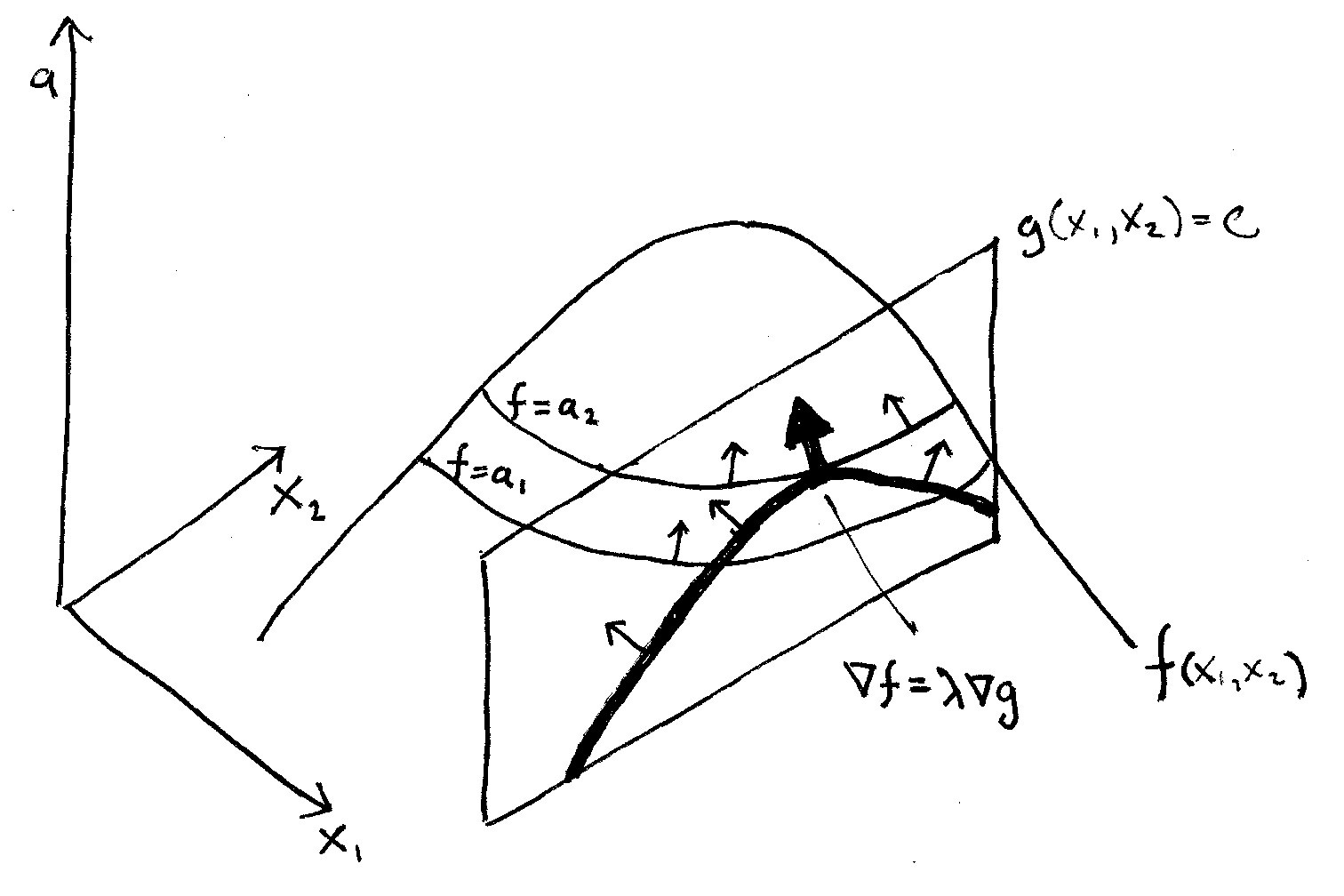
Our goal here is to climb as high on the hill as we can, given that we can?t move any higher than where the constraint g = c cuts the hill.
In the drawing, the boundary where the constraint cuts the function is marked with a heavy line. Along that line are the highest points we can reach without stepping over our constraint. That?s an obvious place to start looking for a constrained maximum.
Imagine hiking from left to right on the constraint line. As we gain elevation, we walk through various level curves of f. I?ve marked two in the picture. At each level curve, imagine checking its slope ? that is, the slope of a tangent line to it ? and comparing that to the slope on the constraint where we?re standing.
If our slope is greater than the level curve, we can reach a higher point on the hill if we keep moving right. If our slope is less than the level curve ? say, toward the right where our constraint line is declining ? we need to move backward to the left to reach a higher point.
When we reach a point where the slope of the constraint line just equals the slope of the level curve, we?ve moved as high as we can. That is, we?ve reached our constrained maximum. Any movement from that point will take us downhill. In the figure, this point is marked with a large arrow pointing toward the peak.
At that point, the level curve f = a2 and the constraint have the same slope. That means they?re parallel and point in the same direction. But as we saw above, gradients are always perpendicular to level curves. So if these two curves are parallel, their gradients must also be parallel.
That means the gradients of f and g both point in the same direction, and differ at most by a scalar. Let?s call that scalar ?lambda.? Then we have,
![]()
Solving for zero, we get
![]()
This is the condition that must hold when we?ve reached the maximum of f subject to the constraint g = c. Now, if we?re clever we can write a single equation that will capture this idea. This is where the familiar Lagrangian equation comes in:
![]()
or more explicitly,
![]()
To see how this equation works, watch what happens when we follow the usual Lagrangian procedure. First, we find the three partial first derivatives of L,
![]()
![]()
![]()
and set them equal to zero. That is, we need to set the gradient of L equal to zero. To find the gradient of L, we take the three partial derivatives of L with respect to x1, x2 and lambda. Then we place each as an element in a 3 x 1 vector. That gives us the following:
Recall that we have two ?rules? to follow here. First, the gradients of f and g must point in the same direction, or
![]()
And second, we have to satisfy our constraint, or
![]()
The first and second elements of the gradient of L make sure the first rule is followed. That is, they force
![]()
assuring that the gradients of f and g both point in the same direction. The third element of the gradient of L is simply a trick to make sure g = c, which is our constraint. In the Lagrangian function, when we take the partial derivative with respect to lambda, it simply returns back to us our original constraint equation.
At this point, we have three equations in three unknowns. So we can solve this for the optimal values of x1 and x2 that maximize f subject to our constraint. And we?re done.
So the bottom line is that Lagrange multipliers is really just an algorithm that finds where the gradient of a function points in the same direction as the gradients of its constraints, while also satisfying those constraints.
As with most areas of mathematics, once you see to the bottom of things ? in this case, that optimization is really just hill-climbing, which everyone understands ? things are a lot simpler than most economists make them out to be.

