Deep learning has caught up very fast with AI enthusiasts and has been spreading like wildfire in the past few years. The number of researchers in the field is growing and more application developers do not want to be left out either. With its growth comes the need to provide different methods and libraries to make it easier and more accessible to everyone. Major programming languages are being introduced while the already existing ones are constantly updated to add deep learning functionalities One of the biggest communities today is the Python community and one of the most popular packages used with python is the NumPy library. In this post, we will look at a brief introduction to the NumPy library and how to use its packages to implement Sigmoid, ReLu and Softmax functions in python. These are the most widely used activation functions in building artificial neural networks for deep learning
Why NumPy?
NumPy is the main package for scientific computations in python and has been a major backbone of Python applications in various computational, engineering, scientific, statistical, image processing, etc fields. NumPy was built from 2 earlier libraries: Numeric and Numarray. [1]Most deep learning algorithms make use of several numpy operations and functions. This is because compared with pure python syntax, NumPy computations are faster. NumPy for instance makes use of vectorization that enables the elimination of unnecessary loops in a code structure, hence reducing latency in execution of code. The following is an example of vectorization for a 1-d array NumPy dot operation, which is mentioned later in the article:
#with vectorizationimport numpy as np #always remember to import numpyimport timet0 = time.process_time()#array1tmatrix1 = [1,2,3,4,5]#array2tmatrix2 = [6,7,8,9,10]#dot matrixnp.dot(tmatrix1,tmatrix2)t1 = time.process_time()print (“dot operation = ” + str(dot) + “n Computation time = ” + str(1000*(t1 – t0)) + “ms”)output: dot operation = 130 Computation time = 0.17037400000008418ms#without vectorizationt0 = time.process_time()dot = 0for i in range(len(tmatrix1)): %time dot+= tmatrix1[i]*tmatrix2[i]t1 = time.process_time()print (“dot operation = ” + str(dot) + “n Computation time = ” + str(1000*(t1 – t0)) + “ms”)output:dot operation = 130 Computation time = 7.590736999999681ms
It can be seen that without vetorizing our code, computation time for a simple loop could be over 40x slower. Now, let?s get back to the basics and see how to do simple numply definitions and operations
Creating vectors and matrices: Vectors (1-d arrays) and matrices (n-d arrays) are among the most basic mathematical data structures used in machine/deep learning learning.
import numpy as np#create a 1-d array of 1,2,3mvector = np.array([1,2,3])print(mvector)output: [1 2 3]#create a 2×3 matrix/2-d arraymmatrix= np.array([[1,2,3],[4,5,6]])print(mmatrix)output: [[1 2 3] [4 5 6]]
Getting properties of a numpy array/matrix
#print array typeprint(type(mmatrix))output: <class ?numpy.ndarray?>#print array shapeprint(mmatrix.shape)output: (2, 3)#print array sizeprint(mmatrix.size)output: 6#print smallest number in a matrixprint(mmatrix.min())output: 1#print biggest numberprint(mmatrix.max())output: 6
Common Mathematical operations
#Adding, subtracting and multiplying#array1mmatrix1 = np.array([[1,2,3],[4,5,6]])#array2mmatrix2 = np.array([[6,7,8],[8,9,10]])#add matricesaddmatrix = np.add(mmatrix1,mmatrix2)print(?addmatrix n?, addmatrix)#subtract matricessubmatrix = np.subtract(mmatrix1,mmatrix2)print(?submatrix n?, submatrix)#multiply matricesmulmatrix = np.multiply(mmatrix1,mmatrix2)print(?mulmatrix n?, mulmatrix)#Calculating dot products#array1dmatrix1 = np.array([[1,2,3],[4,5,6]])#array2dmatrix2 = np.array([[6,7],[8,9],[9,10]])print(?array1 n?, dmatrix1)print(?array2 n?, dmatrix2)#dot matrixdotmatrix = np.dot(dmatrix1,dmatrix2)print(?dotmatrix n?, dotmatrix)#Finding the exponential of a matrixmexp = np.exp(mmatrix)print(mexp)Outputs:addmatrix [[ 7 9 11] [12 14 16]] submatrix [[-5 -5 -5] [-4 -4 -4]] mulmatrix [[ 6 14 24] [32 45 60]]dotmatrix [[ 49 55][118 133]]matrix exponential [[ 2.71828183 7.3890561 20.08553692] [ 54.59815003 148.4131591 403.42879349]]
Common Statistical operations
#print variance of a matrixprint(np.var(mmatrix))output:2.9166666666666665#print mean of a matrixprint(np.mean(mmatrix))output:3.5#print standard deviation of a matrixprint(np.std(mmatrix))output:1.707825127659933
Reshaping Arrays
#Reshape mmatrix from a 2×3 array to a 3×2 arrayrematrix = mmatrix.reshape(3,2)print(rematrix.shape)output:(3, 2)#flatten mmatrix to 1-d arrayflmatrix = mmatrix.flatten()print(flmatrix)output:[1 2 3 4 5 6]
Now let?s define three major activation functions used in deep learning and have a look at simple ways of implementing them with numpy
- The Sigmoid Activation Function
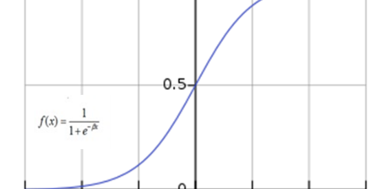
Using a mathematical definition, the sigmoid function [2] takes any range real number and returns the output value which falls in the range of 0 to 1. Based on the convention, the output value is expected to be in the range of -1 to 1. The sigmoid function produces an ?S? shaped curve (figure 1). Mathematically, sigmoid is represented as:
 Equation 1. The Sigmoid function
Properties of the Sigmoid Function
- The sigmoid function takes in real numbers in any range and returns a real-valued output.
- The first derivative of the sigmoid function will be non-negative (greater than or equal to zero) or non-positive (less than or equal to Zero).
- It appears in the output layers of the Deep Learning architectures, and is used for predicting probability based outputs and has been successfully implemented in binary classification problems, logistic regression tasks as well as other neural network applications.
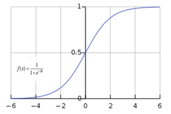 figure 1. The sigmoid function produces as ?S? shape
Now let?s see how to easily implement sigmoid easily using numpy
#sigmoid functiondef sigmoid(X): return 1/(1+np.exp(-X))#Example with mmatrix defined abovesigmoid(mmatrix)output:array([[0.73105858, 0.88079708, 0.95257413], [0.98201379, 0.99330715, 0.99752738]])
2. ReLu
The Rectified linear unit (ReLu) [3] activation function has been the most widely used activation function for deep learning applications with state-of-the-art results. It usually achieves better performance and generalization in deep learning compared to the sigmoid activation function.
Properties of the ReLu Function
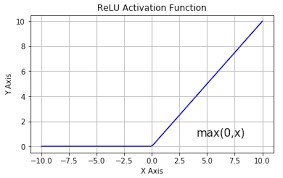
- The main idea behind the ReLu activation function is to perform a threshold operation to each input element where values less than zero are set to zero (figure 2).
Mathematically it is defined by:
 Equation 2. The ReLu function
And is shown as :
Implementing the ReLu function in NumPy is very straight forward:
#ReLu functiondef relu(X): return np.maximum(0,X)#Example with mmatrix defined aboverelu(mmatrix)output:array([[1, 2, 3], [4, 5, 6]])
3. The Softmax Function
The Softmax function is used for prediction in multi-class models where it returns probabilities of each class in a group of different classes, with the target class having the highest probability. The calculated probabilities are then helpful in determining the target class for the given inputs.
Properties of the Softmax Function
- The Softmax function produces an output which is a range of values between 0 and 1, with the sum of the probabilities been equal to 1.
- The Softmax function is computed using the relationship:
 Equation 3. The Softmaxfunction
- The main difference between the Sigmoid and Softmax functions is that Sigmoid is used in binary classification while the Softmax is used for multi-class tasks
Softmax in NumPy:
#softmax functiondef softmax(X): expo = np.exp(X) expo_sum = np.sum(np.exp(X)) return expo/expo_sum#Example with mmatrix defined aboveprint (softmax(mmatrix))output: [[0.00426978 0.01160646 0.03154963] [0.08576079 0.23312201 0.63369132]]
Summary
This post is an introduction to simple NumPy operations and provides a guide to writing simple activation functions common in deep learning using the numpy package. For more information, you may visit the NumPy official website (https://www.numpy.org).
If you liked this post, kindly CLAP and FOLLOW ME for more future posts. All comments are welcome
Bibliography
[1] [Online]. Available: https://www.numpy.org/devdocs/about.html.[2] C. M. Jun Han, ?The influence of the sigmoid function parameters on the speed of backpropagation learning,? in From Natural to Artificial Neural Computation, 1995. [3] R. S. M. A. M. R. J. D. &. H. S. S. Richard H. R. Hahnloser, ?Digital selection and analogue amplification coexist in a cortex-inspired silicon circuit,? Nature, vol. 405, p. 947?951, 2000.
[4] Goodfellow, Bengio & Courville 2016, pp. 183?184:

