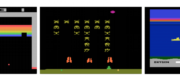
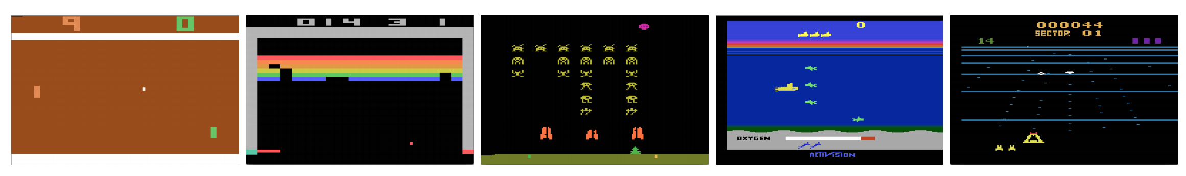
 Atari game
Can computers play video games like a human? In 2015, DQN beat human experts in many Atari games. But once comes to complex war strategy games, AI does not fare well. In 2017, a professional team beat a DeepMind AI program in Starcraft 2 easily.
As quoted from the DeepMind paper:
It is a multi-agent problem with multiple players interacting; there is imperfect information due to a partially observed map; it has a large action space involving the selection and control of hundreds of units; it has a large state space that must be observed solely from raw input feature planes; and it has delayed credit assignment requiring long-term strategies over thousands of steps.
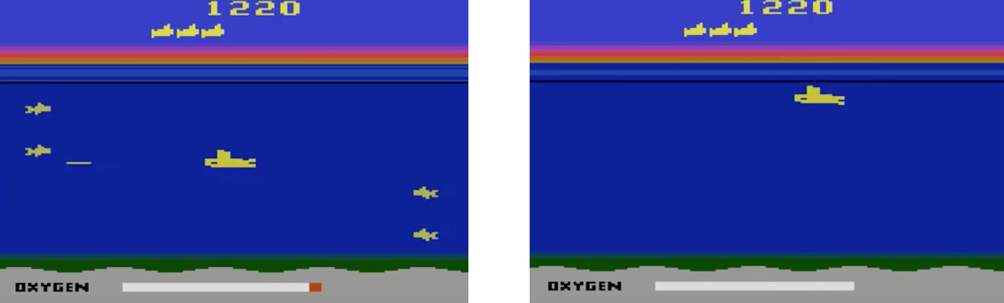
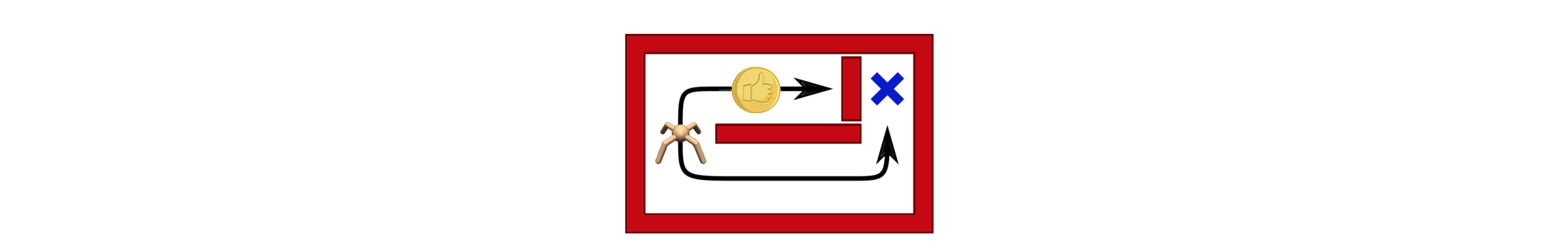
Let?s restart our journey back to the Deep Q-Network DQN. In the Seaquest game below, DQN learns how to read scores, shoot the enemy, and rescue divers from the raw images, all by itself. It also discovers knowledge that we may refer as a strategy, like, when to bring the submarine to the surface for oxygen.
Q-learning learns the action-value function Q(s, a): how good to take an action at a particular state. For example, for the board position below, how good to move the pawn two steps forward. Literally, we assign a scalar value over the benefit of making such a move.
Q is called the action-value function (or Q-value function in this article).
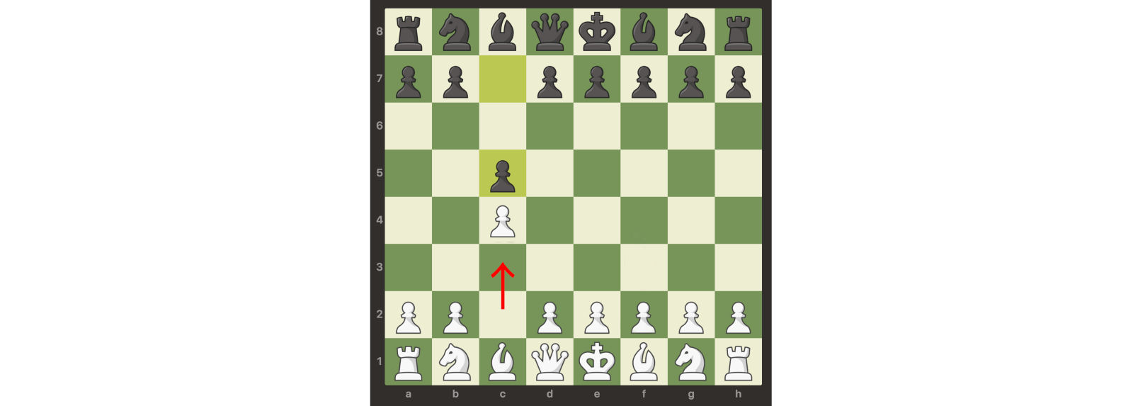
In Q-learning, we build a memory table Q[s, a] to store Q-values for all possible combinations of s and a. If you are a chess player, it is the cheat sheet for the best move. In the example above, we may realize that moving the pawn 2 steps ahead has the highest Q values over all others. (The memory consumption will be too high for the chess game. But let?s stick with this approach a little bit longer.)
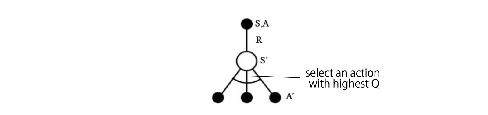
Technical speaking, we sample an action from the current state. We find out the reward R (if any) and the new state s? (the new board position). From the memory table, we determine the next action a? to take which has the maximum Q(s?, a?).
 source
In a video game, we score points (rewards) by shooting down the enemy. In a chess game, the reward is +1 when we win or -1 if we lose. So there is only one reward given and it takes a while to get it.
Q-learning is about creating the cheat sheet Q.
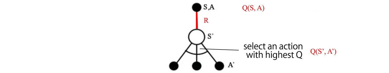
We can take a single move a and see what reward R can we get. This creates a one-step look ahead. R + Q(s?, a?) becomes the target that we want Q(s, a) to be. For example, say all Q values are equal to one now. If we move the joystick to the right and score 2 points, we want to move Q(s, a) closer to 3 (i.e. 2 + 1).

As we keep playing, we maintain a running average for Q. The values will get better and with some tricks, the Q values will converge.
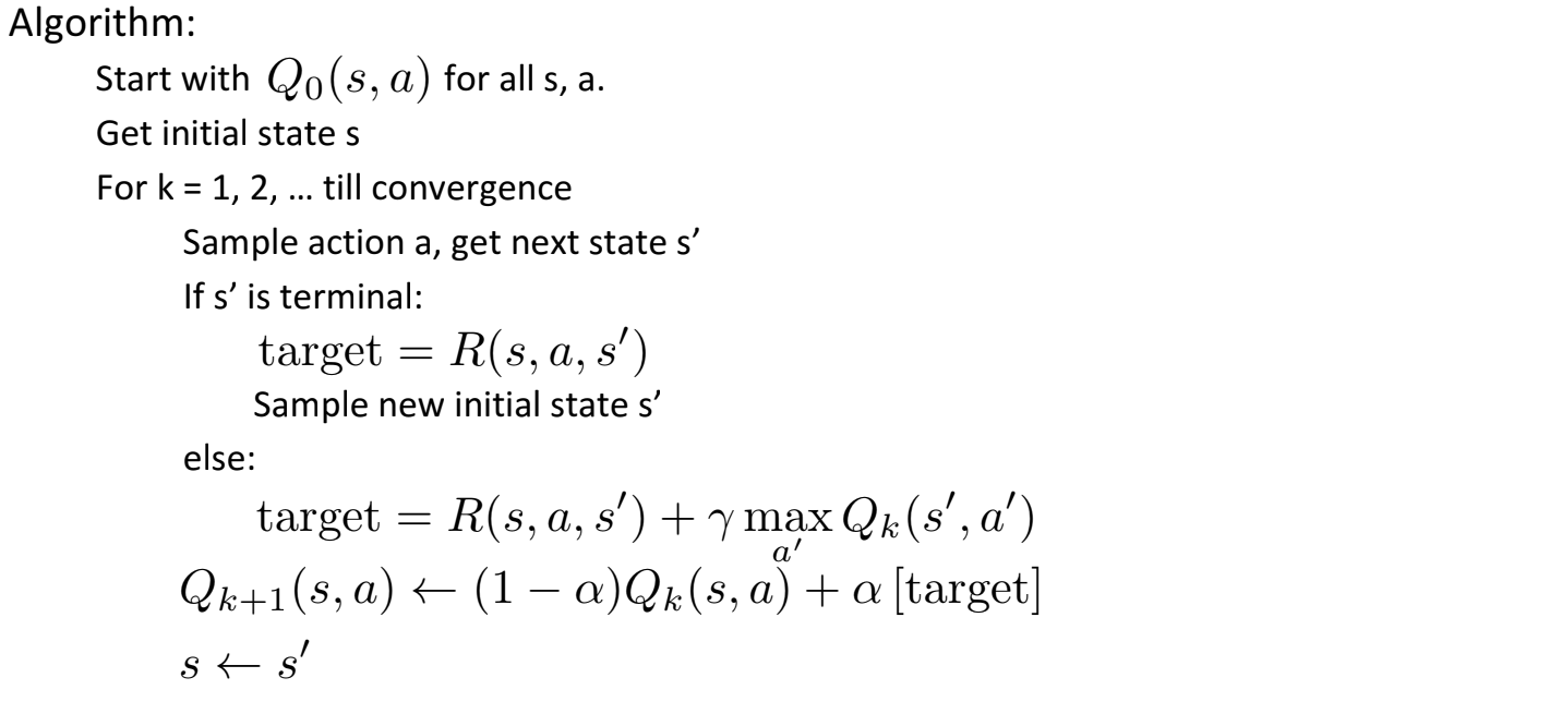
Q-learning algorithm
The following is the algorithm to fit Q with the sampled rewards. If ? (discount factor) is smaller than one, there is a good chance that Q converges.
 Source
However, if the combinations of states and actions are too large, the memory and the computation requirement for Q will be too high. To address that, we switch to a deep network Q (DQN) to approximate Q(s, a). The learning algorithm is called Deep Q-learning. With the new approach, we generalize the approximation of the Q-value function rather than remembering the solutions.
What challenges does RL face comparing to DL?
In supervised learning, we want the input to be i.i.d. (independent and identically distributed), i.e.
- Samples are randomized among batches and therefore each batch has the same (or similar) data distribution.
- Samples are independent of each other in the same batch.
If not, the model may be overfitted for some class (or groups) of samples at different time and the solution will not be generalized.
In addition, for the same input, its label does not change over time. This kind of stable condition for the input and the output provides the condition for the supervised learning to perform well.
In reinforcement learning, both the input and the target change constantly during the process and make training unstable.
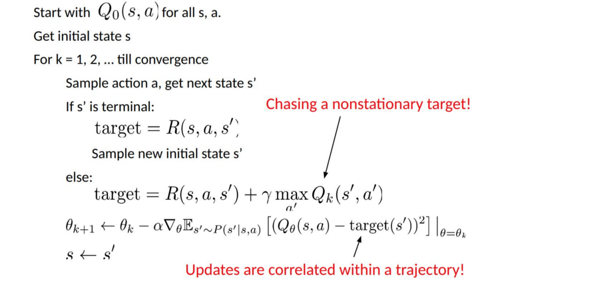
Target unstable: We build a deep network to learn the values of Q but its target values are changing as we know things better. As shown below, the target values for Q depends on Q itself, we are chasing a non-stationary target.
 Source
i.i.d.: There is another problem related to the correlations within a trajectory. Within a training iteration, we update model parameters to move Q(s, a) closer to the ground truth. These updates will impact other estimations. When we pull up the Q-values in the deep network, the Q-values in the surrounding states will be pulled up also like a net.

Let?s say we just score a reward and adjust the Q-network to reflect it. Next, we make another move. The new state will look similar to the last one in particular if we use raw images to represent states. The newly retrieved Q(s?, a?) will be higher and our new target for Q will move higher also regardless of the merit of the new action. If we update the network with a sequence of actions in the same trajectory, it magnifies the effect beyond our intention. This destabilizes the learning process and sounds like dogs chasing their tails.
What is the fundamental challenge in training RL? In RL, we often depend on the policy or value functions to sample actions. However, this is frequently changing as we know better what to explore. As we play out the game, we know better about the ground truth values of states and actions. So our target outputs are changing also. Now, we try to learn a mapping f for a constantly changing input and output!
Luckily, both input and output can converge. So if we slow down the changes in both input and output enough, we may have a chance to model f while allowing it to evolve.
Solutions
Experience replay: For instance, we put the last million transitions (or video frames) into a buffer and sample a mini-batch of samples of size 32 from this buffer to train the deep network. This forms an input dataset which is stable enough for training. As we randomly sample from the replay buffer, the data is more independent of each other and closer to i.i.d.
Target network: We create two deep networks ?- and ?. We use the first one to retrieve Q values while the second one includes all updates in the training. After say 100,000 updates, we synchronize ?- with ?. The purpose is to fix the Q-value targets temporarily so we don?t have a moving target to chase. In addition, parameter changes do not impact ?- immediately and therefore even the input may not be 100% i.i.d., it will not incorrectly magnify its effect as mentioned before.

With both experience replay and the target network, we have a more stable input and output to train the network and behaves more like supervised training.
Experience replay has the largest performance improvement in DQN. Target network improvement is significant but not as critical as the replay. But it gets more important when the capacity of the network is small.
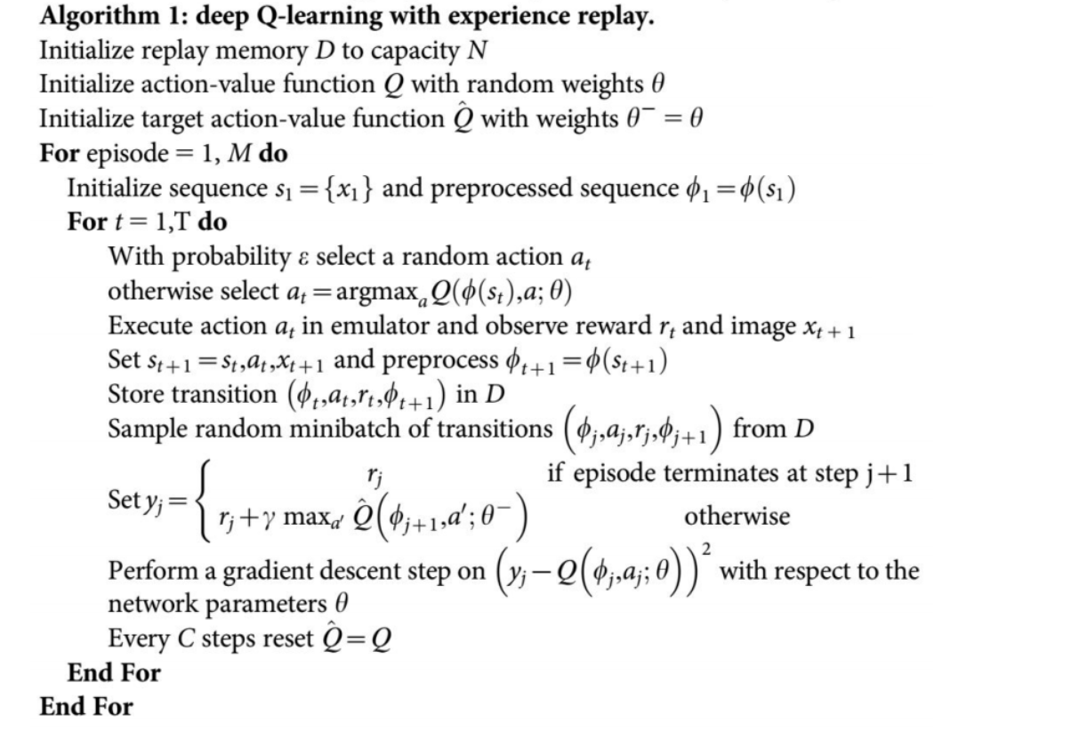
Deep Q-learning with experience replay
Here is the algorithm:
 Source
where ? preprocess last 4 image frames to represent the state. To capture motion, we use four frames to represent a state.
Implementation details
Loss function
Let?s go through a few more implementation details to improve performance. DQN uses Huber loss (green curve) where the loss is quadratic for small values of a, and linear for large values.
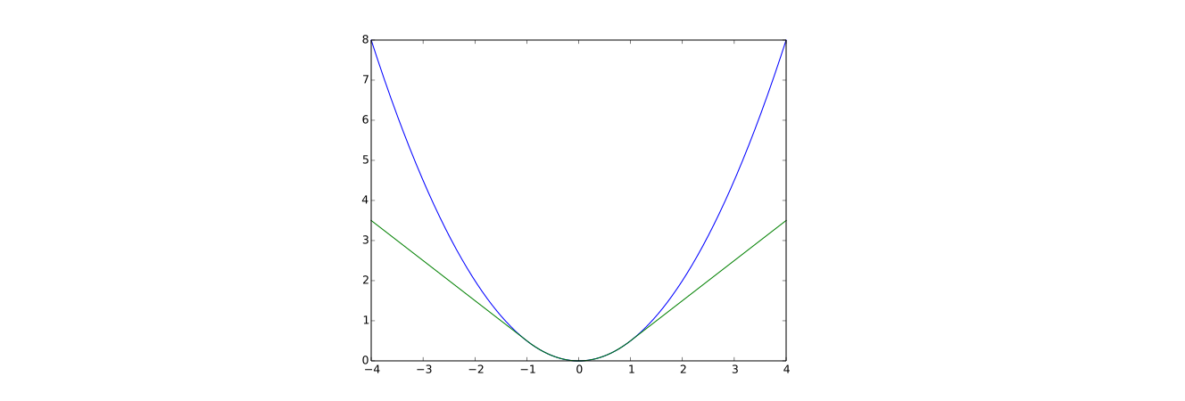 Green is the Huber loss and blue is the quadratic loss (Wikipedia)
The introduction of Huber loss allows less dramatic changes which often hurt RL.
Optimization
RL training is sensitive to optimization methods. Simple learning rate schedule is not dynamic enough to handle changes in input during the training. Many RL training uses RMSProp or Adam optimizer. DQN is trained with RMSProp. Using advance optimization method in Policy Gradient methods is also heavily studied.
?-greedy
DQN uses ?-greedy to select the first action.
 Q-learning: modified from source
To improve the training, ? starts at 1 and anneal to 0.1 or 0.05 over the first million frames using the following policy.

where m is the number of possible actions. At the beginning of the training, we uniformly select possible actions but as the training progress, we select the optimal action a* more frequently. This allows maximum exploration at the beginning which eventually switch to exploitation.
But even during testing, we may maintain ? to a small value like 0.05. A deterministic policy may stuck in a local optimal. A non-deterministic policy allows us to break out for a chance to reach a better optimal.
 Modified from source
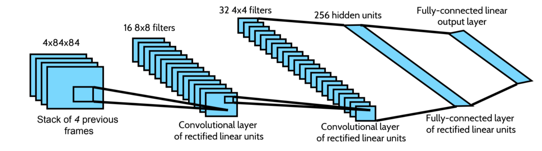
Architecture
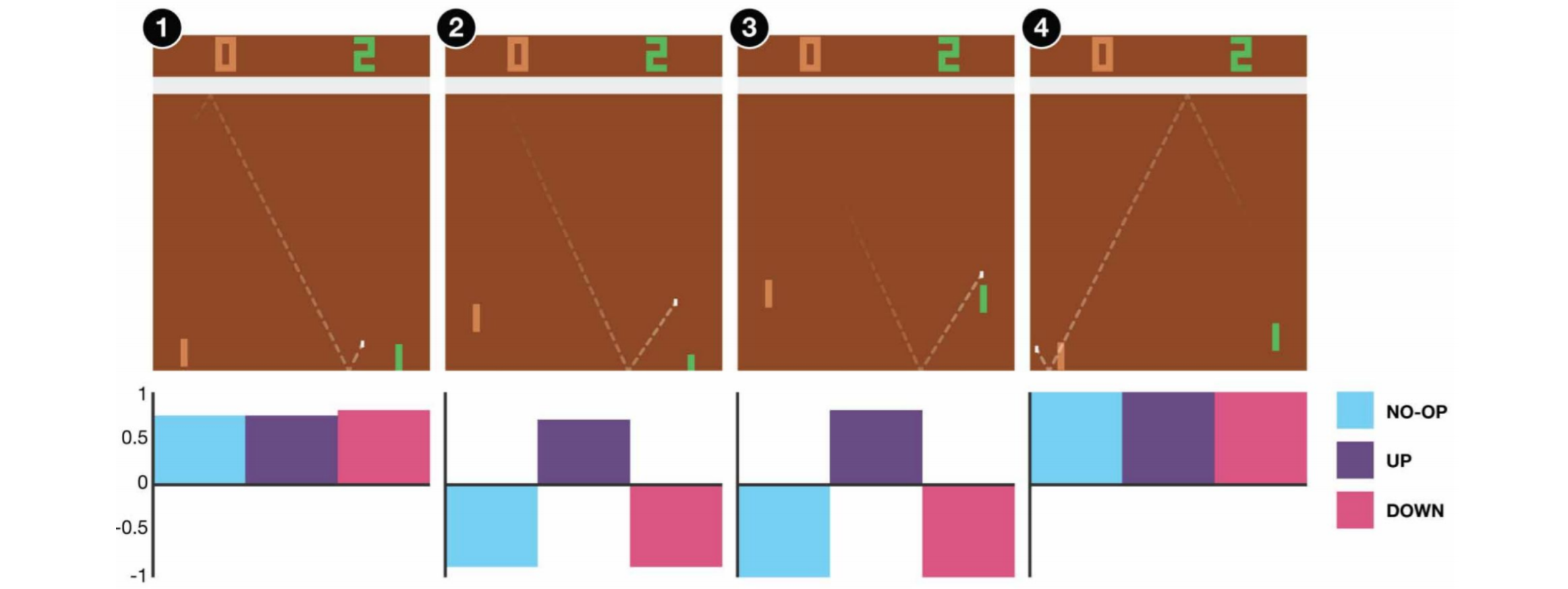
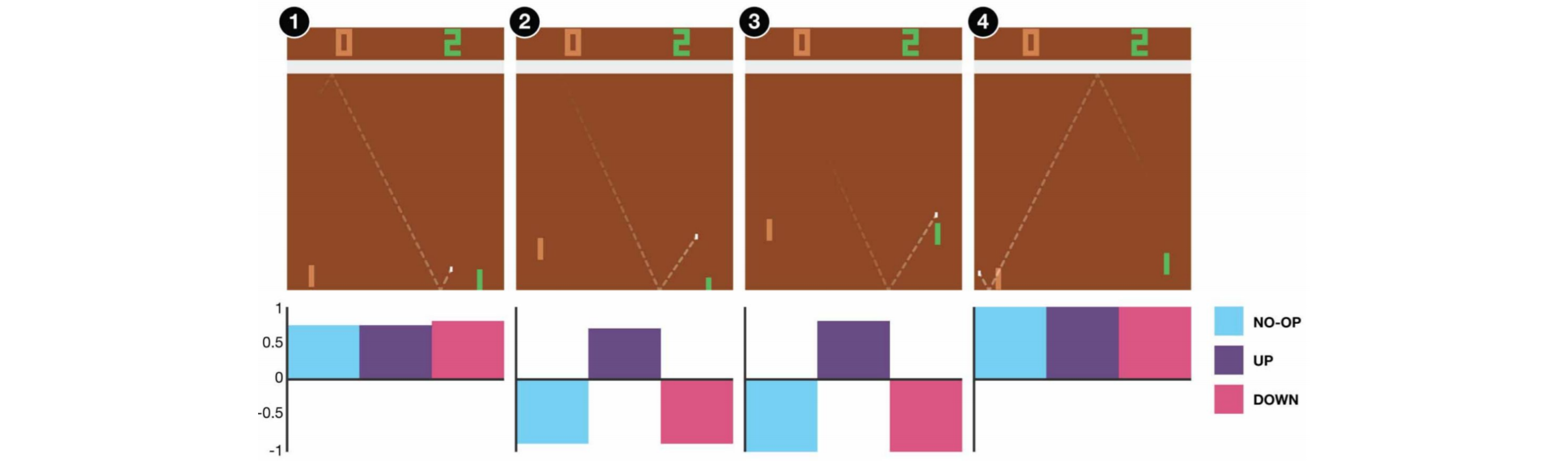
Here is the DQN architecture. We take the last 4 previous video frames and feed them into convolutional layers followed by fully connected layers to compute the Q values for each action.
In the example below, if we do not move the paddle up at frame 3, we will miss the ball. As expected from the DQN, the Q value of moving the paddle up is much higher compared with other actions.
Improvements to DQN
Many improvements are made to DQN. In this section, we will show some methods that demonstrate significant improvements.
Double DQN
In Q-learning, we use the following formula for the target value for Q.

However, the max operation creates a positive bias towards the Q estimations.
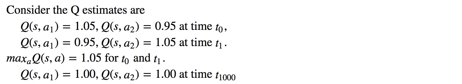
From the example above, we see max Q(s, a) is higher than the converged value 1.0. i.e. the max operation overestimates Q. By theory and experiments, DQN performance improves if we use the online network ? to greedy select the action and the target network ?- to estimate the Q value.

Prioritized Experience Replay
DQN samples transitions from the replay buffer uniformly. However, we should pay less attention to samples that is already close to the target. We should sample transitions that have a large target gap:

Therefore, we can select transitions from the buffer
- based on the error value above (pick transitions with higher error more frequently), or
- rank them according to the error value and select them by rank (pick the one with higher rank more often).
For details on the equations on sampling data, please refer to the Prioritized Experience Replay paper.
Dueling DQN
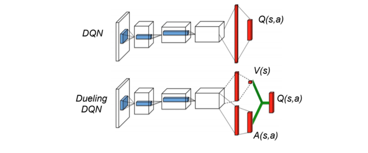
In Dueling DQN, Q is computed with a different formula below with value function V and a state-dependent action advantage function A below:

 Source
Instead of learning Q, we use two separate heads to compute V and A. Empirical experiments show the performance improves. DQN updates the Q-value function of a state for a specific action only. Dueling DQN updates V which other Q(s, a?) updates can take advantage of also. So each Dueling DQN training iteration is thought to have a larger impact.
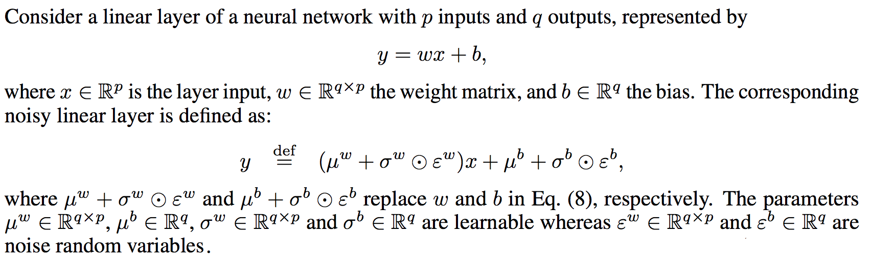
Noisy Nets for Exploration
DQN uses ?-greedy to select actions. Alternatively, NoisyNet replaces it by adding parametric noise to the linear layer to aid exploration. In NoisyNet, ?-greedy is not used. It uses a greedy method to select actions from the Q-value function. But for the fully connected layers of the Q approximator, we add trainable parameterized noise below to explore actions. Adding noise to a deep network is often equivalent or better than adding noise to an action like that in the ?-greedy method.
 Source
More thoughts
DQN belongs to one important class of RL, namely value-learning. In practice, we often combine policy gradients with value-learning methods in solving real-life problems.
Credit and references
UCL Course on RL
UC Berkeley RL Bootcamp
DQN paper
